
Deconvolving Overlapping Chromatography Peaks: A Researcher’s Guide

Deconvolving overlapping chromatography peaks is the process of separating co-eluting or partially overlapping signals into their individual component peaks for accurate quantitation and identification. Standard resolution metrics like the USP resolution equation break down when valley heights exceed roughly 40% of the smaller peak height, making computational separation methods the only reliable path forward. Techniques including Gaussian curve fitting, exponentially modified Gaussian (EMG) modeling, derivative spectral analysis, and physically guided spectral reconstruction each address different overlap scenarios. Selecting the right method requires understanding the data’s signal-to-noise ratio, peak spacing, and intensity ratios before any algorithm is applied.
What causes peaks to overlap in chromatography?
Peak overlap is the direct result of insufficient chromatographic resolution between two or more analytes. Understanding the root cause determines which separation or deconvolution strategy is appropriate.
The most common sources of overlapping peaks include:
- Co-elution from similar retention properties. Structural analogs, enantiomers, and matrix components with near-identical partition coefficients elute within the same retention window, producing fused or shouldered peaks.
- Column saturation and overloading. Injecting too much sample mass causes peak broadening and asymmetric tailing, which pushes adjacent peaks into each other even when they would otherwise be resolved.
- Instrument band broadening. Extra-column volume from injector dead volume, connecting tubing, and detector cell geometry adds variance to every peak. This broadening is additive and narrows the effective resolution between closely spaced analytes.
- Method limitations. Gradient programs optimized for one analyte class often compress or expand retention windows for others, creating localized overlap in complex matrices.
The analytical consequences are significant. Overlapping peaks distort peak area integration, inflate or suppress quantitative results, and can mask minor components entirely. Traditional integration software assigns a single apex to what is actually a composite signal, producing systematic error in concentration calculations. When the valley between two peaks rises above approximately 40% of the smaller peak’s height, classic resolution equations no longer yield reliable estimates. At that point, the valley-height method or full computational deconvolution becomes necessary.
What are the core deconvolution techniques for overlapping peaks?
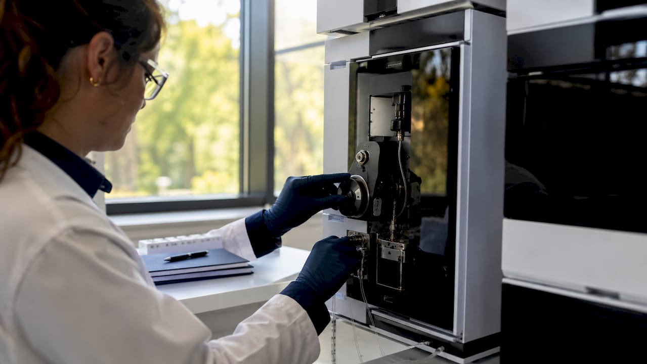
No single deconvolution method works across all overlap scenarios. Method selection depends on peak energy spacing, intensity ratios, and the signal-to-noise characteristics of the dataset.
The four principal approaches are:
-
Mathematical peak fitting. Gaussian, Lorentzian, Voigt, and EMG models are fitted to the composite signal using nonlinear least-squares algorithms. Each model assumes a specific peak shape. The EMG model is the most physically realistic for chromatographic peaks because it accounts for the exponential tailing caused by mass transfer kinetics. Fitting quality is assessed using residual plots and F-statistics to confirm that added peaks improve the model significantly.
-
Derivative-based spectral separation. Computing the second or fourth derivative of the chromatogram sharpens peak features and reveals shoulders invisible in the raw signal. The method works because differentiation suppresses broad baseline contributions while amplifying narrow peak features. The critical limitation is noise amplification. Derivative operations amplify high-frequency noise, so the signal must be denoised and smoothed before differentiation is applied.
-
Physically guided spectral reconstruction. This approach applies hard constraints derived from ultra-high-resolution reference data to guide the fitting of low-resolution chromatographic signals. Combining physical constraints with mathematical models overcomes the underdetermined nature of purely statistical fitting, producing solutions that are both mathematically convergent and physically defensible. This technique is particularly effective in hyphenated systems like LC-DAD or GC-MS where spectral libraries provide the constraint information.
-
Advanced computational algorithms for multidimensional data. In comprehensive two-dimensional chromatography (GC×GC-TOFMS), algorithms like 2D mzCompare apply mass spectral matching across the full two-dimensional retention space. 2D mzCompare resolves over 95% of components at low saturation and 62% at higher saturation, while reducing effective 2D peak widths by approximately 12-fold. That 12-fold gain in resolution density is transformative for complex mixture analysis.
Pro Tip: When fitting EMG or Voigt models, always examine the residual plot for systematic patterns. Random residuals confirm a good model fit; structured residuals indicate a missing peak component or an incorrect shape assumption.
What preprocessing steps are required before deconvolution?
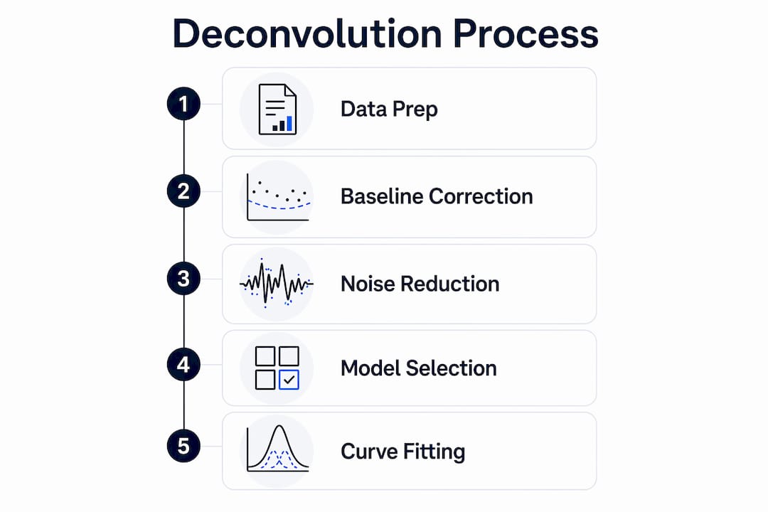
Preprocessing is not optional. Deconvolution applied to uncorrected data produces results that are mathematically plausible but analytically meaningless.
The required preparatory steps are:
- Baseline correction. Drift, solvent gradients, and detector noise create a non-zero baseline that shifts peak positions and distorts area calculations. Subtracting a fitted baseline before any peak modeling removes this systematic artifact. Polynomial, spline, and asymmetric least-squares methods each suit different baseline morphologies.
- Denoising. Robust noise handling requires strict preprocessing in the sequence: denoising, interpolation, then differentiation. Reversing this order introduces edge artifacts and amplifies noise into the derivative domain.
- Peak tracking and assignment. Correctly assigning peaks across multiple conditions or samples is the foundation of any multi-condition deconvolution model. Peak tracking is the critical bottleneck in chromatographic modeling and must be verified manually before mathematical fitting begins.
- Calibration alignment. Standards and samples must be processed under identical mathematical transformations. Any asymmetry in preprocessing between the calibration set and the unknown introduces proportional error into the final quantitative result.
Pro Tip: Apply baseline correction and denoising in a reproducible scripted workflow rather than interactively. Interactive adjustments introduce operator-dependent variability that cannot be audited or replicated.
How to execute deconvolution step by step
A structured workflow prevents the most common sources of error and produces results that can be validated against independent criteria.
-
Acquire and inspect raw data. Examine the chromatogram for baseline stability, noise level, and the number of visible shoulders or inflection points. Count the minimum number of component peaks required to explain the composite signal shape.
-
Apply preprocessing. Perform baseline correction, denoising, and interpolation in that order. For derivative-based approaches, apply smoothing before differentiation. Document every parameter used.
-
Select the deconvolution method. Use mathematical fitting for well-resolved shoulders with known peak shapes. Use derivative analysis for rapid screening of peak number in low-noise data. Use physically guided reconstruction when spectral library data is available. Use advanced algorithmic tools for multidimensional or mass spectrometric datasets.
-
Fit the model and apply constraints. Initialize peak parameters from derivative analysis or visual inspection. Apply physically meaningful constraints: peak widths must be positive, areas must be non-negative, and retention times must fall within the observed composite peak window.
-
Validate the result. Check residuals for systematic patterns. Confirm peak identities using spectral signatures, retention time standards, or spiked reference compounds. For quantitative work, verify recovery using a standard addition experiment.
The table below summarizes which method suits each data scenario:
| Data scenario | Recommended method |
|---|---|
| Two partially overlapping Gaussian peaks, low noise | EMG or Gaussian curve fitting |
| Multiple shoulders in a complex matrix chromatogram | Derivative analysis for peak counting, then fitting |
| LC-DAD or GC-MS with spectral library available | Physically guided spectral reconstruction |
| GC×GC-TOFMS high-complexity mixture | 2D mzCompare or equivalent algorithmic approach |
| Unknown peak count, moderate noise | Derivative screening followed by constrained fitting |
What common mistakes occur during peak deconvolution?
Most deconvolution failures trace back to a small set of identifiable errors, each with a specific remedy.
- Noise amplification in derivative methods. Applying differentiation to insufficiently smoothed data produces spurious inflection points that are misinterpreted as real peaks. The fix is to denoise before differentiating and to verify candidate peaks against the raw signal.
- Assuming perfect peak symmetry at low concentrations. At trace levels, detector noise dominates the peak wings, making EMG tailing parameters unreliable. Fixing the tailing factor from a high-concentration calibration standard and applying it to the trace-level fit produces more defensible results.
- Fitting without selective unoverlapped regions. Peaks lacking selective windows yield models that converge mathematically but carry no physical meaning. Before trusting any automated fitting output, verify that at least one component has a region of the chromatogram where it contributes signal without interference from other components.
- Peak misassignment across conditions. In multi-condition experiments, a peak that shifts retention time may be assigned to the wrong component in one run. Peak identity misassignment invalidates the entire deconvolution model for that condition. Cross-check assignments using spectral matching or spiked standards.
- Overreliance on automated outputs. Automated deconvolution software reports a result for every dataset it receives. The result is only meaningful if the preprocessing, model selection, and constraint choices were appropriate. Expert review of residuals and spectral signatures remains non-negotiable.
Key Takeaways
Deconvolving overlapping chromatography peaks requires rigorous preprocessing, method-matched fitting models, and expert validation of residuals and spectral signatures before any quantitative result can be trusted.
| Point | Details |
|---|---|
| Method selection is data-specific | Choose fitting, derivative, or reconstruction methods based on signal-to-noise ratio and peak spacing. |
| Preprocessing determines result quality | Baseline correction, denoising, and peak tracking must be completed before any fitting is applied. |
| Selective regions anchor physical meaning | Verify that at least one component has an unoverlapped signal region before trusting automated outputs. |
| Derivative methods amplify noise | Always denoise and smooth before differentiation to prevent spurious peak detection. |
| Validation is mandatory | Confirm deconvolution results using residual analysis, spectral matching, and spiked reference standards. |
Why I think most labs underestimate the preprocessing problem
After working through a substantial number of chromatographic deconvolution problems, the pattern I see most consistently is not a failure of the algorithm. It is a failure of the data going into the algorithm. Researchers reach for sophisticated fitting software before they have corrected the baseline, verified peak tracking, or confirmed that their smoothing parameters are appropriate for the noise level in their specific detector. The algorithm then produces a confident-looking result on flawed input.
The physically guided spectral reconstruction approach impresses me most as a direction for the field. Anchoring a mathematical fit to hard constraints from high-resolution reference spectra is the right instinct. It forces the model to produce a physically defensible answer rather than just a numerically convergent one. The 2D mzCompare results in GC×GC-TOFMS, where algorithmic approaches reduce 2D peak widths by approximately 12-fold, show what is possible when the algorithm is designed around the physics of the measurement.
My caution is against treating deconvolution as a black box. Automated tools are genuinely useful, but they require a researcher who understands what the residuals mean and can recognize when a mathematically valid fit is physically implausible. The combination of rigorous preprocessing, appropriate model selection, and expert residual review is what separates publishable results from numerical artifacts.
— Nadeem
R2nsoftware PeakLab for chromatographic peak resolution
Researchers who need to move from manual fitting workflows to a validated computational environment will find R2nsoftware’s PeakLab platform purpose-built for this work. PeakLab supports up to 1,000 simultaneous peaks with Gaussian, Lorentzian, Voigt, and EMG models, integrated baseline correction, and F-statistic-based model validation. The platform handles both single-dimension chromatographic data and hyphenated spectral datasets within the same environment.

For researchers working with automated signal detection across large sample sets, R2nsoftware’s AutoSingal applies automated peak detection and deconvolution with reproducible parameter sets, reducing operator-dependent variability across batches. Both tools integrate directly with existing chromatography data systems and support export formats compatible with standard laboratory reporting workflows.
FAQ
What is peak deconvolution in chromatography?
Peak deconvolution is the computational process of separating a composite chromatographic signal into its individual component peaks. It applies mathematical models such as Gaussian, EMG, or Voigt functions to extract peak area, height, and retention time for each overlapping analyte.
When should I use derivative analysis instead of curve fitting?
Use derivative analysis when you need to count the number of peaks in a composite signal before fitting, or when the peak shapes are unknown. Use curve fitting once the peak count and approximate shape model are established.
Why do my deconvolution results look correct but fail validation?
The most common cause is the absence of selective unoverlapped regions for one or more components. Models without selective windows converge mathematically but lack physical meaning. Verify that each fitted component has at least one region where it contributes signal without interference.
How does preprocessing affect deconvolution accuracy?
Preprocessing determines the quality of every result that follows. Denoising, baseline correction, and calibration must be applied in the correct sequence before any derivative or fitting operation is performed.
What is the best method for GC×GC-TOFMS peak overlap?
Algorithmic approaches designed for two-dimensional retention space, such as 2D mzCompare, are the most effective. These methods resolve over 95% of components at low saturation levels and reduce effective 2D peak widths by approximately 12-fold compared to standard integration.