Gaussian, Lorentzian, and Pure Voigt Peak Fitting for UV/VIS, IR/FTIR, NIR/FTNIR Spectra
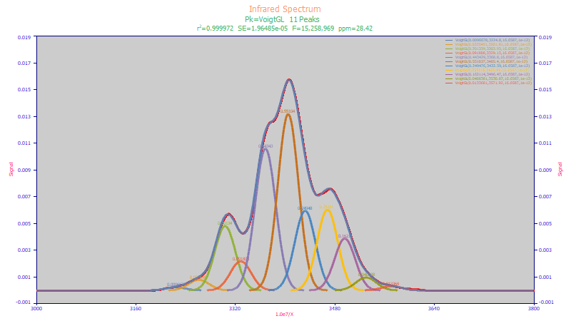
Spectral absorbances often involve heavily convoluted overlapping peaks. PeakLab’s full precision analytical Voigt function is one of 46 built-in spectroscopy functions which is used in the above peak fit to separate individual IR spectral components.
True Voigt Deconvolution
Fitting a true Voigt function will automatically deconvolve the separate Lorentzian and Gaussian components of each spectral peak.
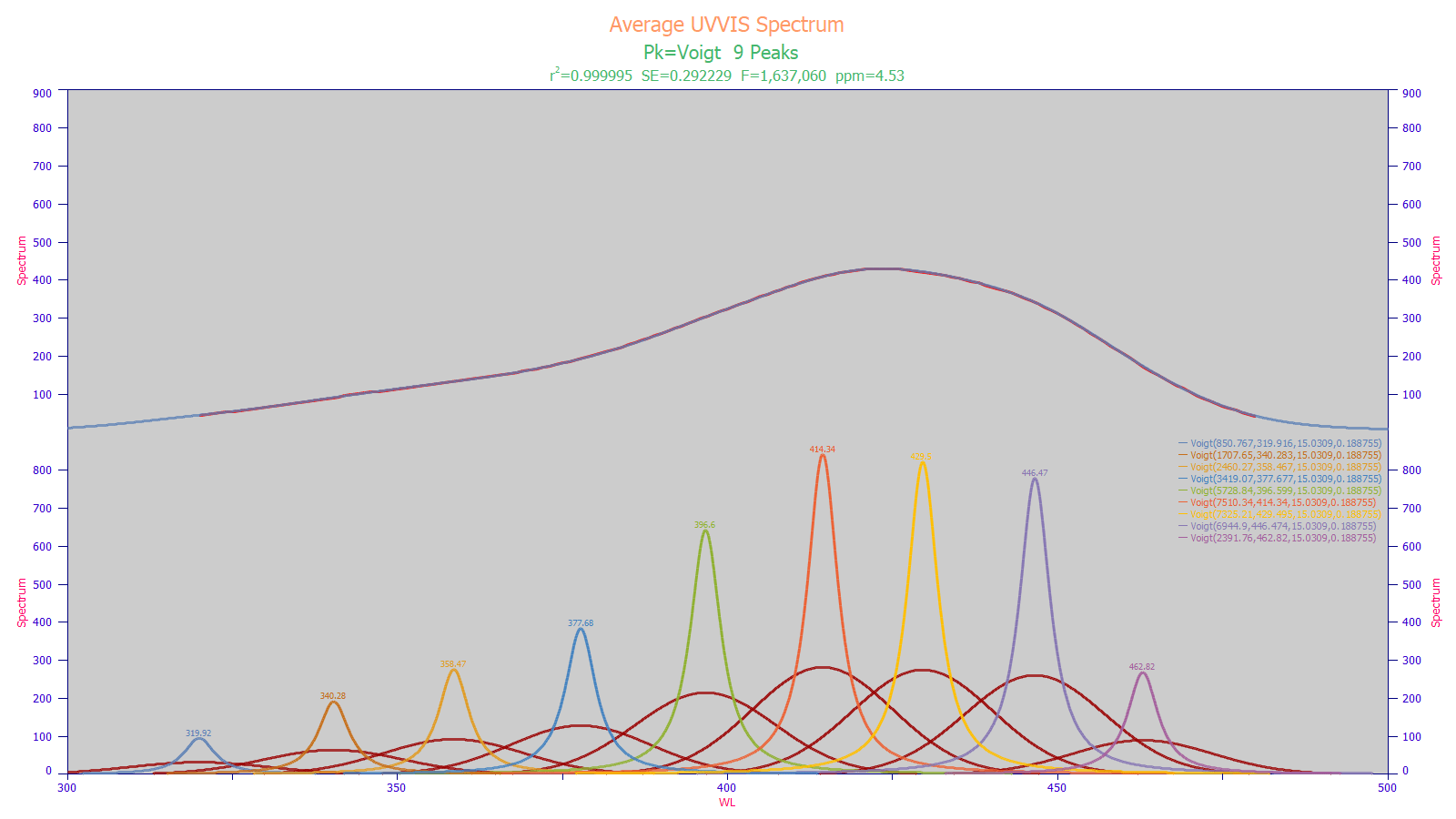
In the above optimum UV-VIS fit, a nine-Voigt model fits the data with a variance error of just 4.5 ppm and an F-statistic of 1.6 million. The deconvolved Lorentzian spectral peaks are those that would be seen in a perfect instrument with no signal smearing from the Gaussian instrument response function, shown in red for each peak. An optimized Voigt fit such as this reveals the principal wavelengths that will be seen by an effective chemometric modeling system.
Voigt Models with IRFs for Asymmetric XPS and Raman Peaks
XPS and Raman spectral peaks generally have an intrinsic asymmetry that can be effectively fit with Voigt models containing instrument response functions.
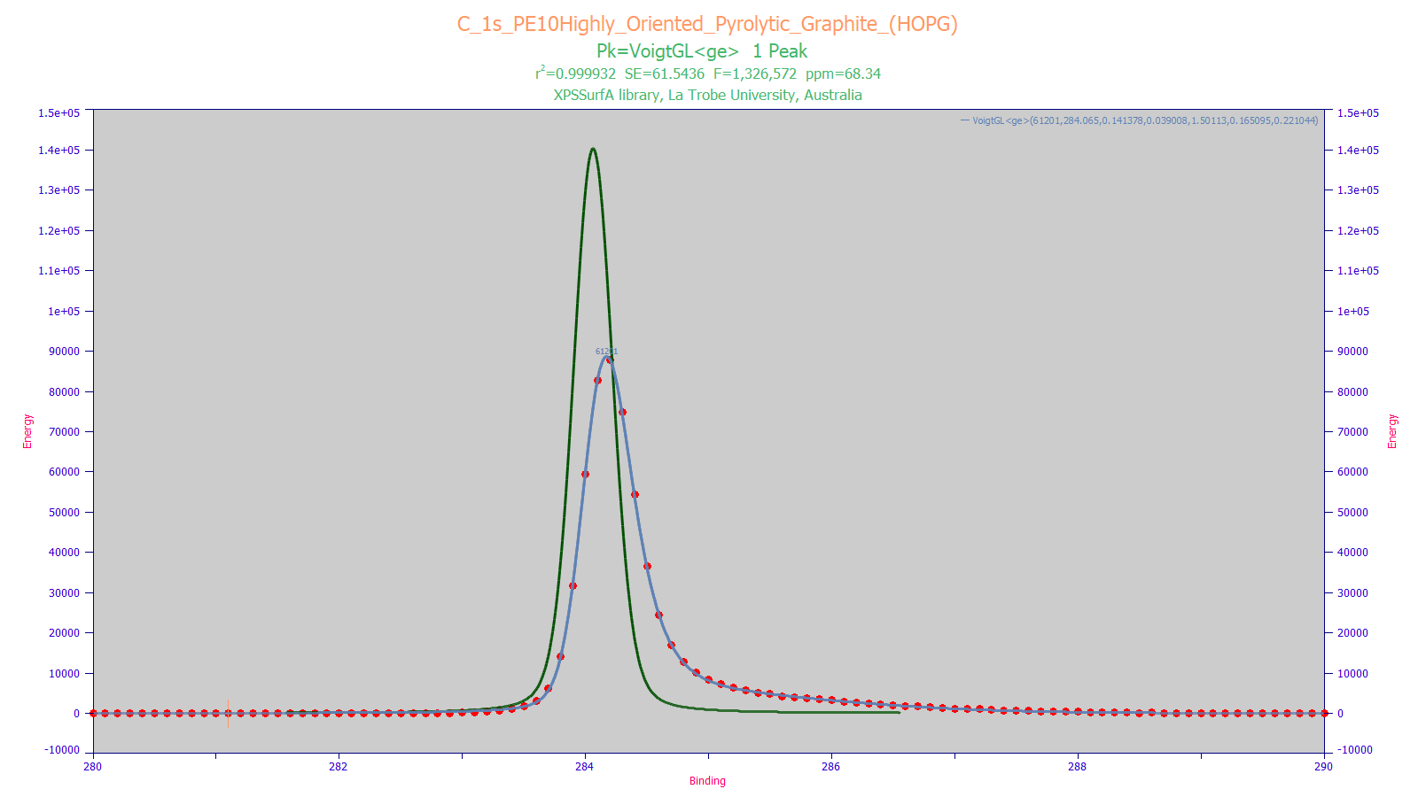
The XPS peak shape above is fitted to a Voigt with an IRF consisting of a sum of the simplest probability and kinetic distortions. In the above figure, the red points are the raw data, the blue curve is the peak fit, and the green peak is the deconvolved Voigt with the asymmetric distortion removed.
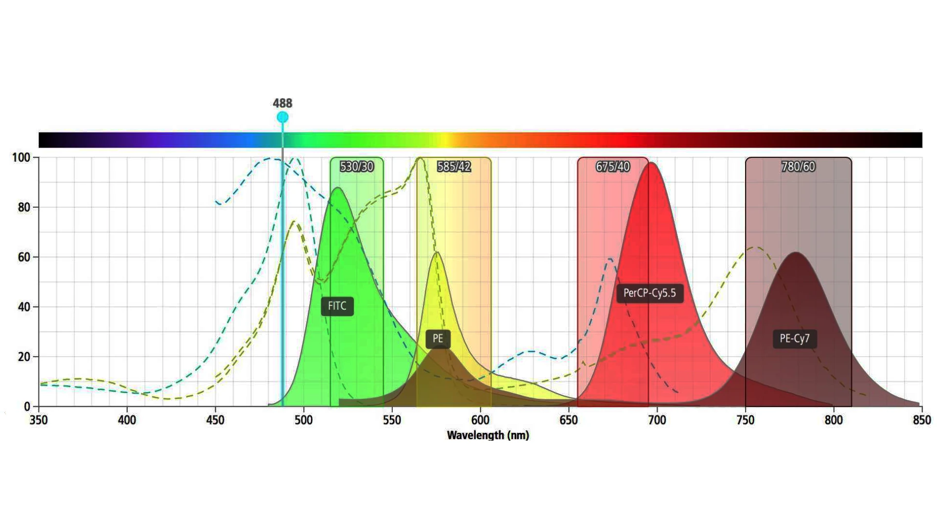
Fluorescence Spectroscopy
Fluorescence excitation and emission spectra can be complex with highly convoluted absorbances. Often a simple multiple-Gaussian model suffices to capture the principal excitation and emission wavelengths.
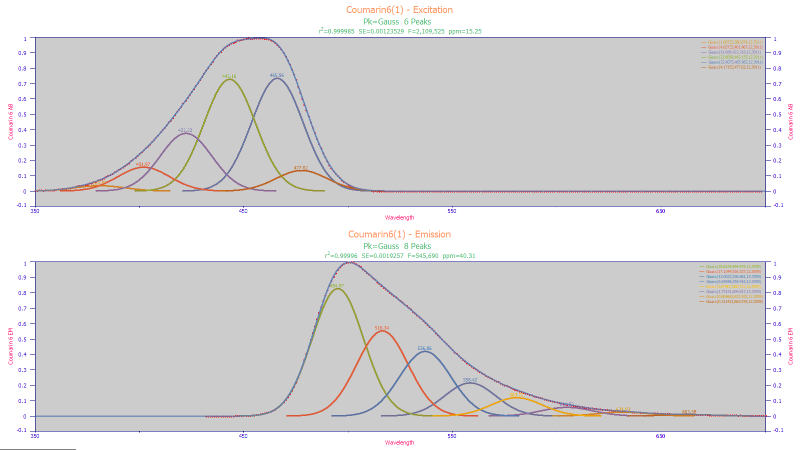
The above are Coumarin 6 excitation and emission spectra. Note the unusual shapes of the overall excitation and emission curves.
Chemometric Predictive Modeling of Spectroscopy Data
PeakLab introduces a new and innovative chemometric modeling solution that is an attractive alternative to the traditional PLS and PCR modeling. These are direct spectral models that outperform the PLS and PCR ‘unscrambling’ algorithms for predictive accuracy and web-based computational performance. These predictive models for spectroscopy are far simpler to understand and exceedingly easy to code and evaluate.
High Accuracy Chromatographic Peak Fitting for System Suitability and QC of Columns and Flow Systems
When you want to know with certainty the state of a column’s health, you need to measure the theoretical plates of just the column’s separation, not artifacts of injectors, detector cells, or changes in the fluid flow path.
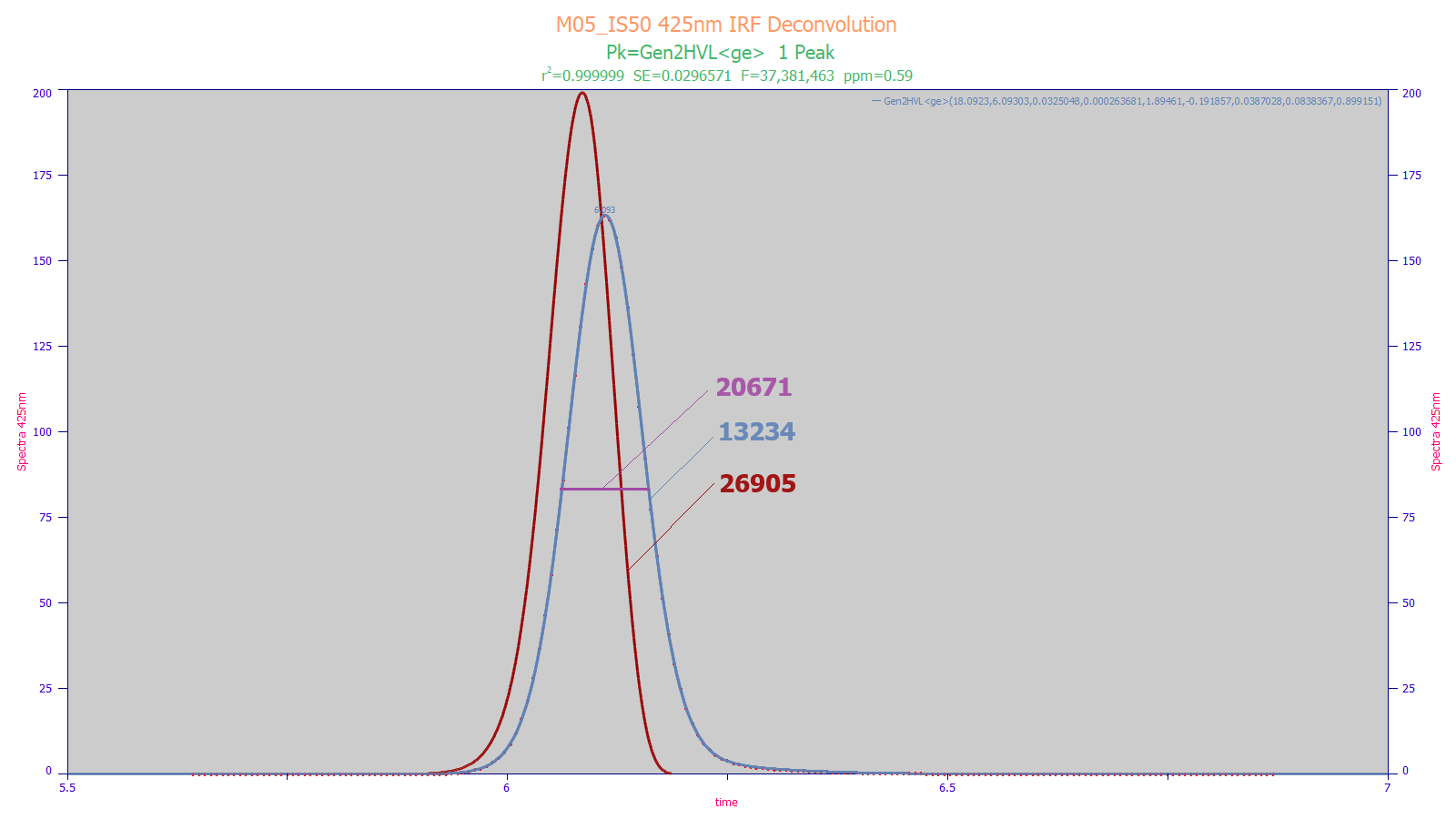
PeakLab fits chromatographic peaks to near perfect goodness of fit values. In the above UHPLC C18 peak fit, the 0.59 ppm unaccounted variance equates to a r2 goodness of fit greater than 0.999999, allowing separation of the column peak from all instrumental distortions. In the fit above, the blue is the observed peak, the red is the peak specific to the column separation minus all instrumental effects. The FWHM traditional Gaussian estimate of N uses only the magenta half-width and produces an N=20,671. The moment method accounts the full blue peak, but that includes the instrumental effects and tailing, and this results in N=13,234. The red deconvolved peak consists of only the column separation minus the instrumental distortions, N=26,905.
PeakLab goes one step further offering a model-based N which removes higher moment differences. such as those which can arise from the packing variation in narrow diameter columns and other nonidealities. For the above peak, the model-based N=35,137, the value that would be seen if the packing and interphase mass transfer were perfectly uniform.
Quantifying the instrument response function (IRF) parameters has value as well. The IRF parameters will catch aging injectors, flow path changes, and differences in detectors. Identifying the IRF also assists in designing preps that minimize these instrumental distortions, such as the differences in mobile phase solvents.
High Accuracy Chromatographic Modeling of Overlapping Peaks – Don’t Reconfigure or Reformulate!
PeakLab introduces two model-based innovations to realize close to perfect fits of real-world chromatographic peaks. The first is the convolution integral fitting of IRFs, and the second is advanced HVL-based models with higher moment statistical generalizations. Both expertly manage the real-world non-idealities of chromatographic peaks.
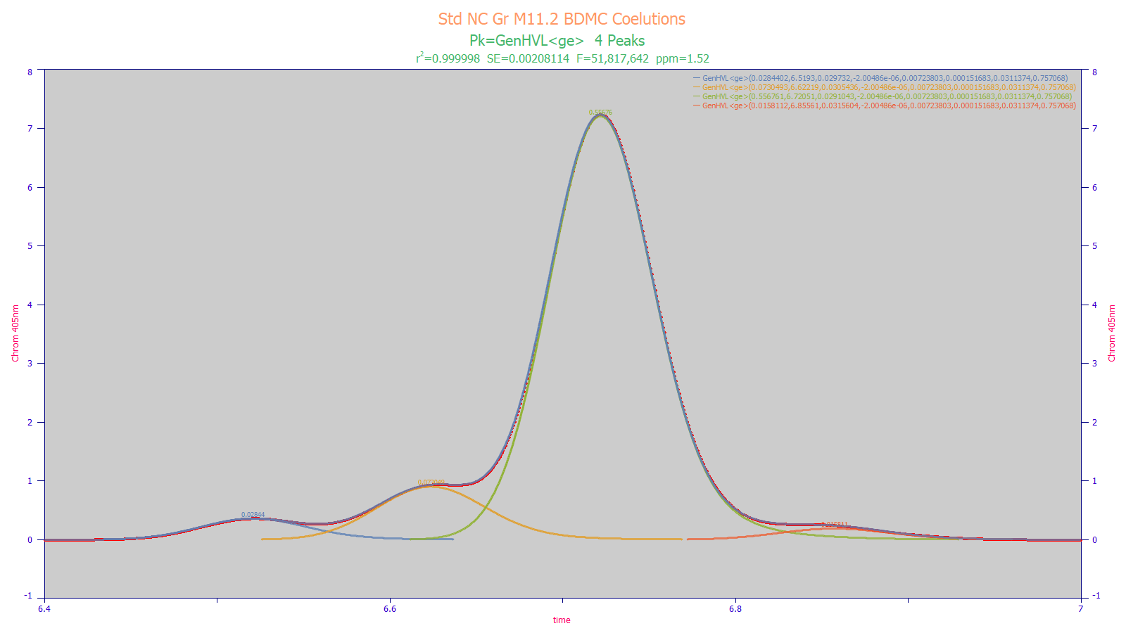
The above separation represents an optimal separation of the BDMC region in a curcuminoid analysis. In most published studies, only a single peak is seen at this location. In this optimized separation, there are three additional components and little prospect for realizing baseline resolved peaks, gradient or isocratic. Despite sharing the tailing-fronting factor and third moment asymmetry across all four peaks, the peak fit above produced an unaccounted variance error of just 1.52 ppm, and accurate estimates of the areas of the four components. PeakLab was also able to process the 3D DAD data to extract and confirm different UV-VIS curcuminoid spectra for the four components. For chromatographic researchers where baseline resolved peaks are not always an option, PeakLab is an indispensable analytical tool.
The new PeakLab modeling of chromatographic peaks is so accurate, you can fit overlapping peaks with separate widths for each peak if just the upper 30% of a peak’s amplitude is exposed on each side, and you can successfully fit any set of overlapping peaks with shared widths and tailing-fronting factors if the second derivative method can simply detect the peak’s presence in the data.
For R&D work, there is no need to reformulate or redesign a separation in order to get baseline-resolved peaks and their conventional integrated areas. As in the example above, highly accurate areas are possible with overlapping peaks.
Gradient UHPLC Reverse-Phase C18 Chromatographic Separations
Gradient UHPLC and HPLC separations add one more tier of complexity to the peak shape. While a third moment adjustment of the underlying density is generally needed for isocratic analytic peaks, gradient peaks require both third and fourth moment adjustments for truly effective modeling as well as an estimate of the aggregate gradient that is present during the analyte’s overall transit through the column.
While a well-crafted gradient can sometimes cancel most of the tailing of the IRF, the compressed shape of a gradient peak still requires this additional fourth moment level of modeling with respect to peak shape. Further, simply because a gradient can cancel much of an IRF, doesn’t mean that this will occur for even a single peak, and it will definitely not occur for peaks which partially or fully transit during an isocratic hold. The IRF will also still be present if a slower gradient is used or if the flow path has a strong IRF that cannot be fully offset by the gradient.
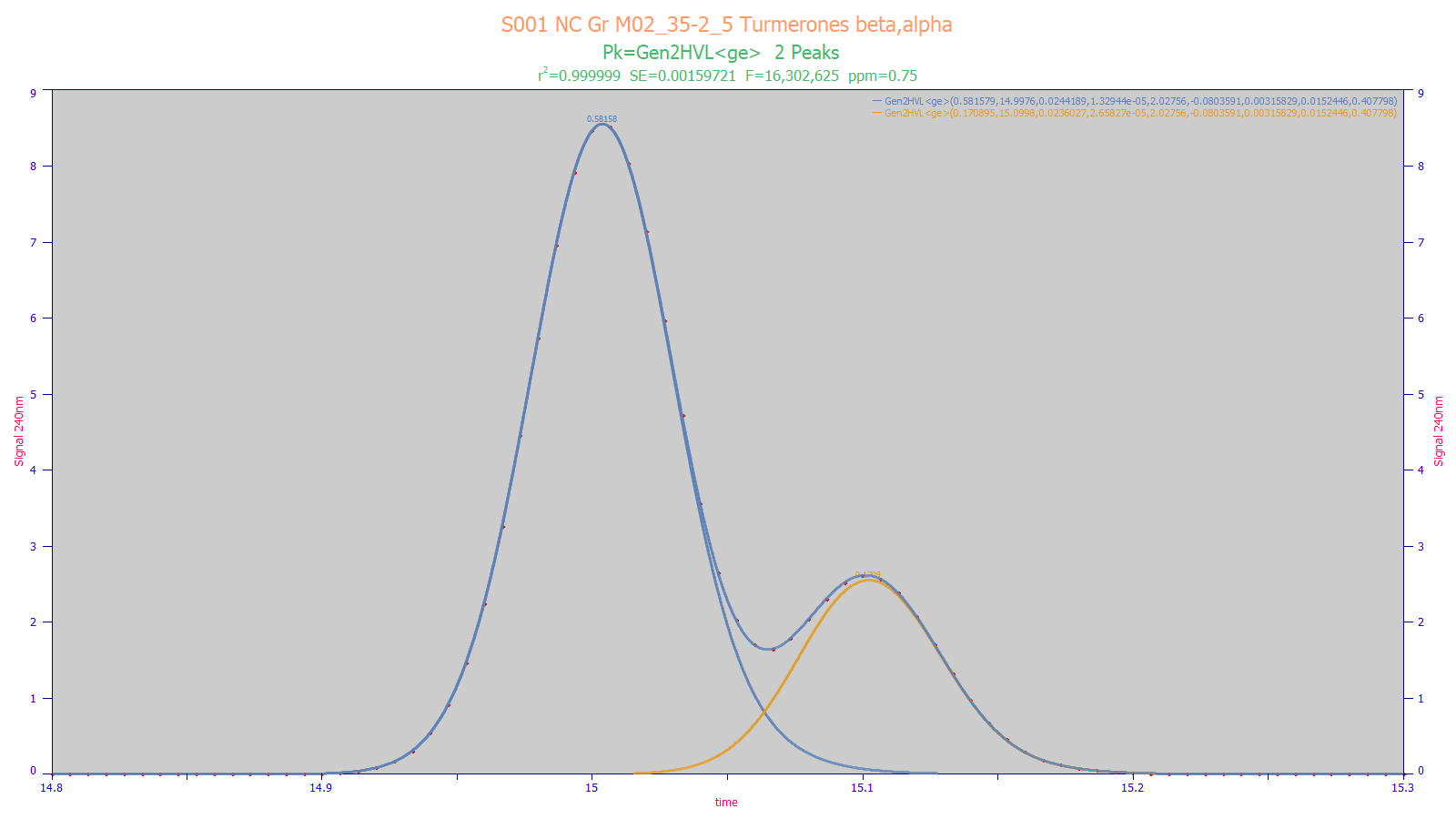
The above gradient peaks consist of near coeluting beta and alpha turmerones. A twice-generalized HVL model with third and fourth moment adjustments and also fitting the non-cancelled portion of the IRF produces a 0.75 ppm unaccounted variance goodness of fit. The modeling was able to fit the peaks to an accuracy which would match that seen with integrating baseline-resolved peaks.
Thermal Gradient GC
Thermal gradient GC peaks often span a large portion of the region of nonlinear-chromatographic shapes, and can vary from close to symmetric peaks at low concentrations to sharply left and right triangular tailed and fronted shapes at high concentrations. Overlapping peaks are often encountered, especially with natural materials with many components.
While the thermal gradient will generally offset the IRF tailing common to conventional GC, these are gradient peaks which require the third and fourth adjustments of a twice-generalized HVL model as well as fitting that is capable of successfully processing small concentration peaks independently. PeakLab has a number of intelligent fit strategies that make even these difficult fits quite easy to realize.
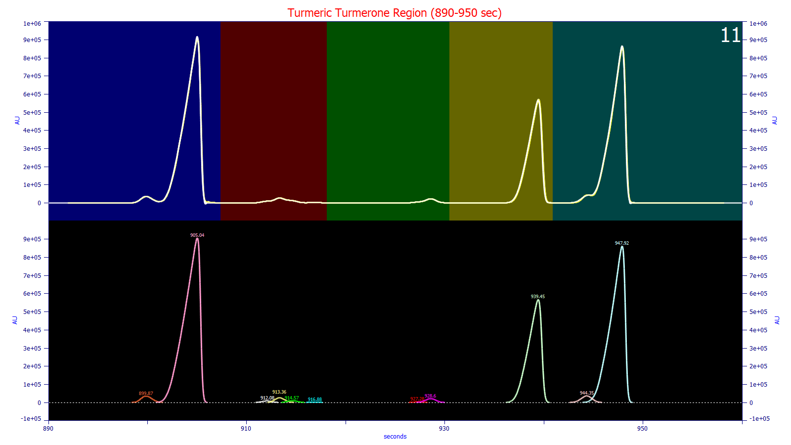
In the above fit of the peaks in the turmerone elution regime of turmeric, the colors in the upper plot represent different data regions in the baseline segments option. This procedure is used to isolate the baseline resolved regions of the elution and independently fit the different overlapping peaks in each segments In each of these fits, the individual peaks in an overlap feature are further fitted individually to better realize the global or optimal fit. In the 62 ppm error fit shown above, PeakLab fit the individual regions separately, each segment sharing the width but varying the tailing-fronting factor. If you look closely, you will see small, close to symmetric peaks in the left tail of the sharply fronted first and third principal turmerone peaks.
Preparative Chromatography
Preparative separations often operate at or beyond the level of column overload. In such a case, you will want to closely monitor the health of the columns.
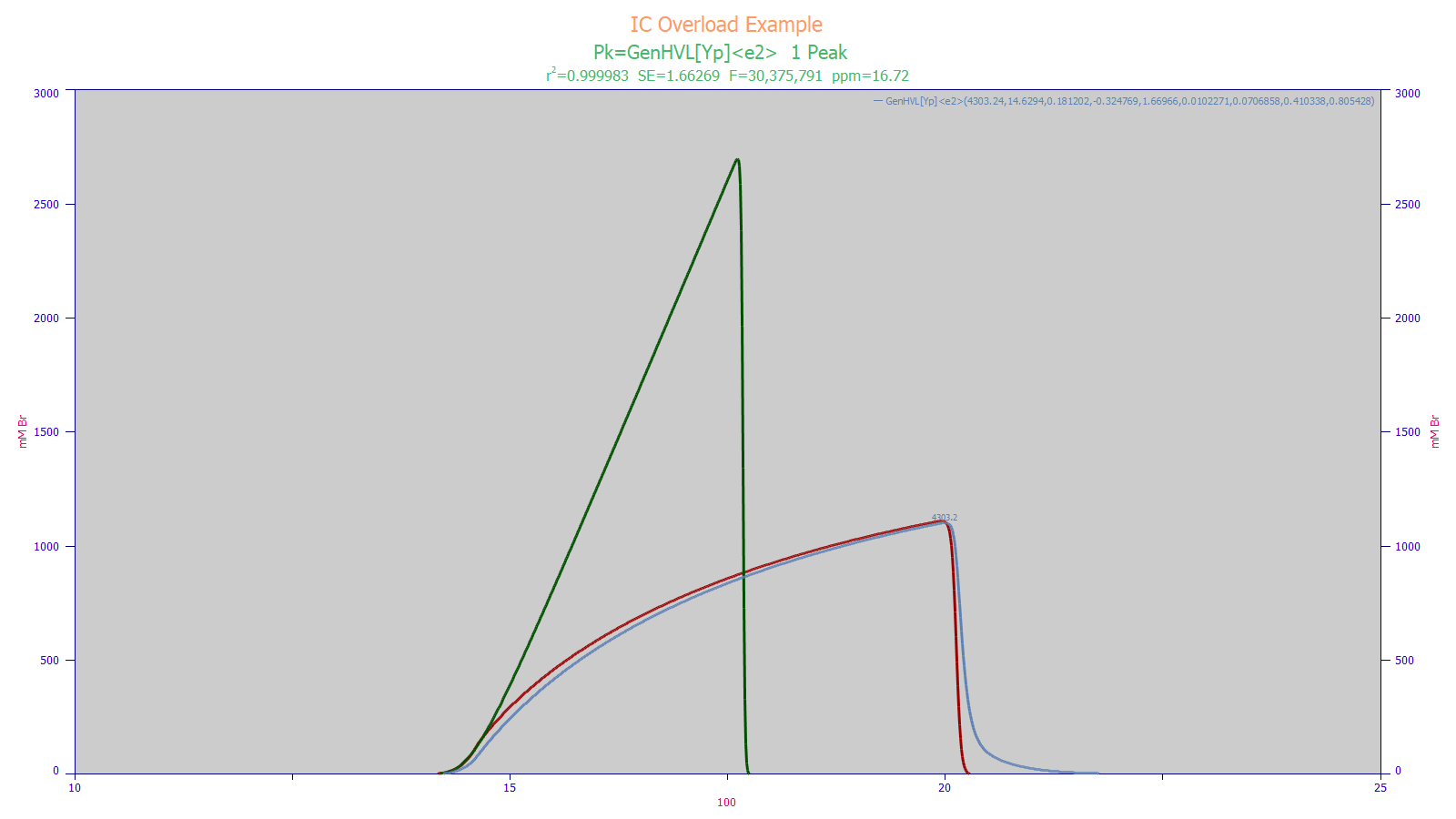
In the above IC preparative separation, the overload state within the column is apparent. The blue curve is the peak as registered by the instrument, the red curve is the peak that would be seen if there were no instrumental distortions, and the green curve is the pure HVL that would be seen if there were no higher moment nonidealities and if the column’s capacity had been such no overload occurred. For the peak as registered by the instrument, the blue curve, the N by the Gaussian FWHM was 125, and the N by moments was 150. For the parametric model where the overload state was deconvolved, the green curve, the separation that would be seen in the column had infinite capacity, N=6518, essentially the value one would expect to see in an analytic separation.
High Speed, Small Column Diameter Separations
If you are working with fast separations using small diameter columns, you are likely to see overlapping peaks, prominent IRFs, and a considerable third moment skew and possibly significant fourth moment dilation.
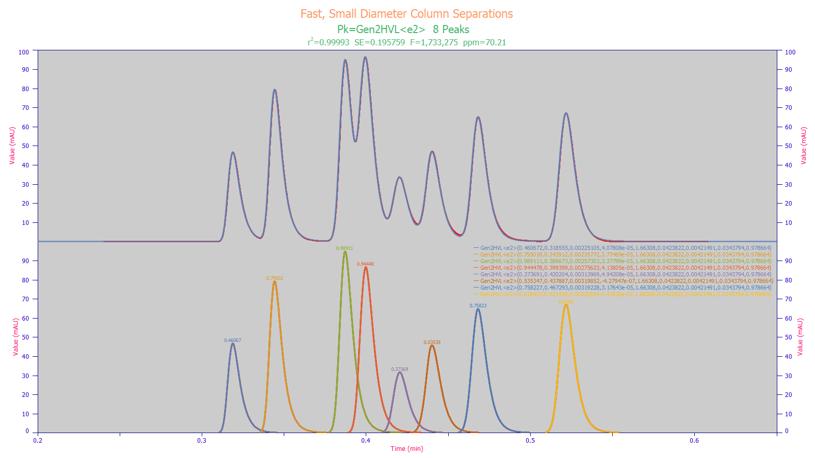
In the above research chromatogram, only one of the eight peaks is baseline resolved where one would see an accurate quantification using conventional integration. PeakLab’s fitting not only accurately determines the areas and center of mass locations of all eight peaks, but it also quantifies the IRF of the instrument as well as the higher moment nonidealities in the separation. When you see peaks such as the above, the brief time required for a PeakLab analysis will give you more analytic information than you would see in an elaborate optimization of the separation where all peaks were baseline resolved.
Chemometric Predictive Modeling of Chromatography with Spectroscopy Data
Chromatographic measurements can be time consuming and costly, and for certain lower accuracy, high-speed screening applications, it may be of value to build a predictive model based on mapping chromatographic analysis values to UV/VIS, IR, FTIR, FTNIR, or other rapid spectroscopic measurements.
PeakLab introduces an innovative chemometric modeling solution that is an attractive alternative to traditional PLS and PCR modeling. These are direct spectral models that outperform the PLS and PCR ‘unscrambling’ algorithms for predictive accuracy and web-based computational performance.
State of the Art Peak Fitting and Direct Spectral Modeling
PeakLab uniquely offers a combination of peak fitting and direct automated multivariate predictive model creation for the most accurate chemometric predictive models you will find in any software product.
The PeakLab predictive modeling is often used to estimate chromatographic or other lab intensive values from far faster and simpler spectroscopy. The PeakLab modeling is a general statistical modeling procedure that can be used for creating a multivariate predictive model from any lab measured value using any data matrix from any source. That matrix series can be spectra in wavelength or frequency, chromatographic data sets in time, or any other collection of data series, including principal components and Fourier domain deconvolved spectra.
A More Accurate and Far Simpler Alternative to PLS and PCR Models
Spectral modeling has largely relied on Partial Least Squares (PLS) or Principal Component Regression (PCR) predictions. Instead of offering one more implementation of these now ubiquitous procedures, we made a conscious choice to produce a wholly new and far simpler robust method for generating these predictive models. If you have used PLS and PCR for chemometric models, please see our analytic reasoning for this new technology near the bottom of this page.
A Complete, Automated, and Simple Chemometric Modeling Solution
The PeakFit solution for chemometric modeling consists of the following:
Visualization For the Detection of outlier Spectra
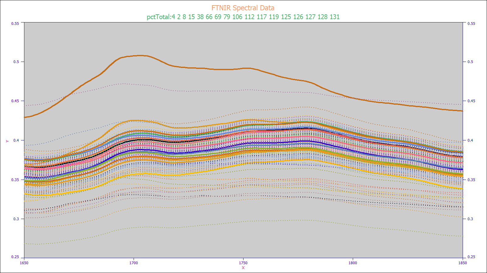
It is not an easy matter to spot an outlier spectrum when plotting hundreds or thousands of spectra that will be fit to produce a predictive model. PeakFit offers a graphical visualization specifically for this task. In the plot below, a data matrix consisting of 156 spectra is plotted and those with a target y value between 4-5% are highlighted.
Peak Fitting for Wavelength And Spectral Resolution
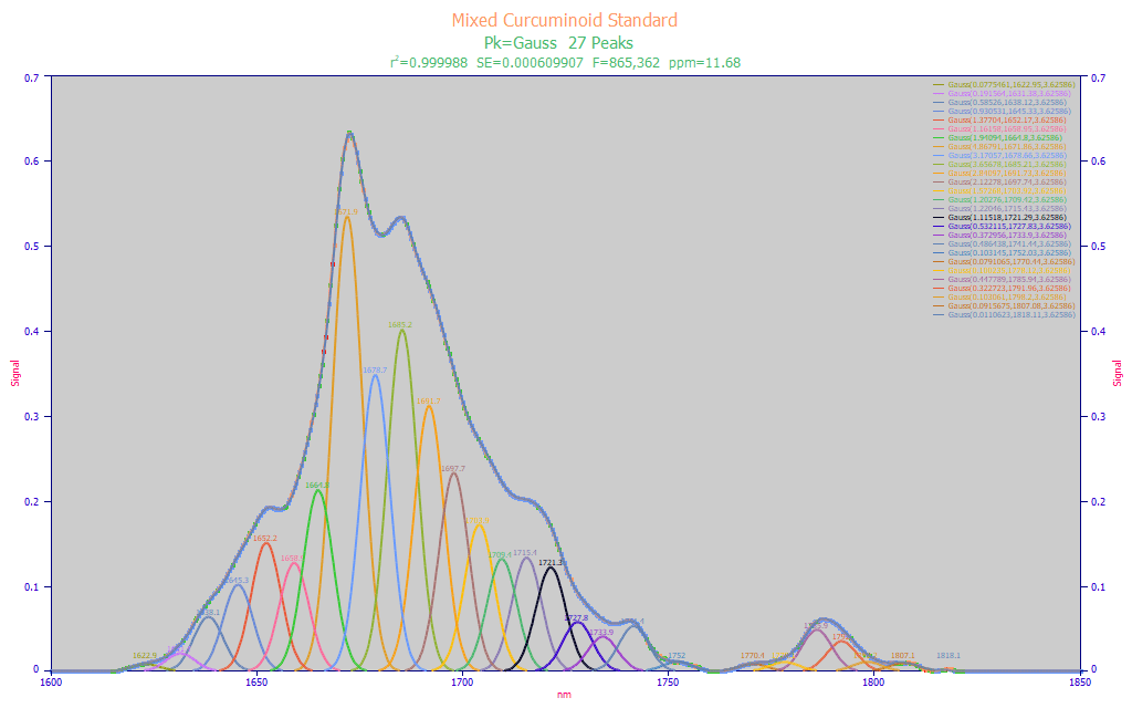
Before building a predictive model, it is useful to fit the spectroscopy for the known target analyte(s) with a set of equal width Gaussian or Voigt peaks. This will furnish two essential pieces of information for the predictive modeling. The optimal fit will determine the spectral resolution of the instrument, and this will be used for setting the x-spacing for the wavelengths in the predictive model. The fitting will also estimate the wavelengths that should appear as the principal predictors in the chemometric models. In the reference standards example below, there are four principal peaks, all at adjacent wavelengths, and the optimal multiple Gaussian fit estimates an SD width of about 4 nm, a reasonable value for high resolution FTNIR spectra.
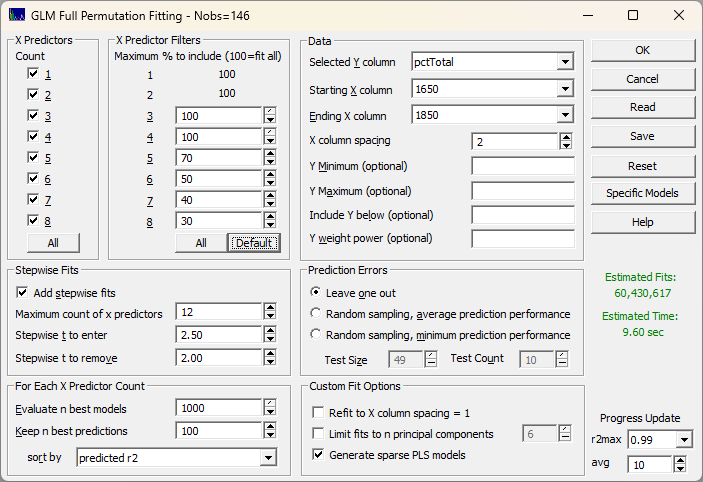
One Click Fitting – One Dialog – Intelligent Expert-System Design
Unlike complex chemometric modeling programs, PeakLab presents the whole of the modeling settings in one dialog where most options can be left at the defaults. Simply select the variable in the data matrix that is to be modeled, the range of the wavelengths you want to use, and use filters, if needed, to produce a reasonable modeling time. In this example, 60 million candidate models will be fit in about 10 seconds. PeakLab’s higher parameter count filters make impractical full permutation fits viable. The fit in the example below would require close to 12 hours and the fitting of 220 billion models without these smart filters that intelligently remove unproductive predictors as the fitting algorithm proceeds.
PeakLab-Specific Smart Stepwise PLS Models
Unique to PeakLab, models with nine and higher parameter counts can be added by a “smart stepwise” procedure that optimally begins with the best retained full permutation fits of a lesser parameter count. The algorithm then uses an intelligent multidimensional search where wavelengths that may have been removed or filtered are given new opportunities to be added back when specific combinations of wavelengths make this possible.
PeakLab-Specific Sparse PLS Models
Also unique to PeakLab are sparse PLS models. These are not partial least squares models formed in the conventional sense, but rather consist of a weighted combination of the best full permutation and stepwise models containing the most statistically significant wavelengths in the retained fitted models. Unlike a PLS model, where every wavelength is weighted into the overall model, these are sparse PLS robust models with up to 15 select wavelengths, all of which are required to test as statistically significant in the individual models that are weighted by prediction goodness of fit into an overall model. Sparse PLS models are a convenience that offer the robustness of combining many different individually effective predictive models across a composite set of deterministic wavelengths.
Full Predictive Modeling Science
PeakLab is founded upon advanced proprietary predictive modeling science developed for financial time series. You should find PeakLab’s predictive modeling to be the most effective commercially available chemometric predictive modeling in the world, but we also believe you will find it is the most accessible, straightforward, and intelligent.
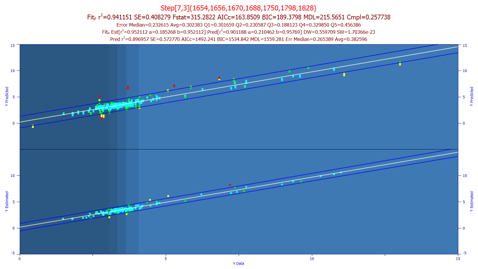
In the above predictive model plots, the x-axis contains known chromatographic reference values and the y-axis contains the prediction from the spectroscopy. The lower plot shows the leave-one-out prediction errors from the selected model where each point is an average of multiple spectral replicates. The upper plot shows the prediction error of out-of-sample spectra (wholly unknown to the model) and where, as in field analyses, no replicates were averaged and individual spectra were used for the estimation.
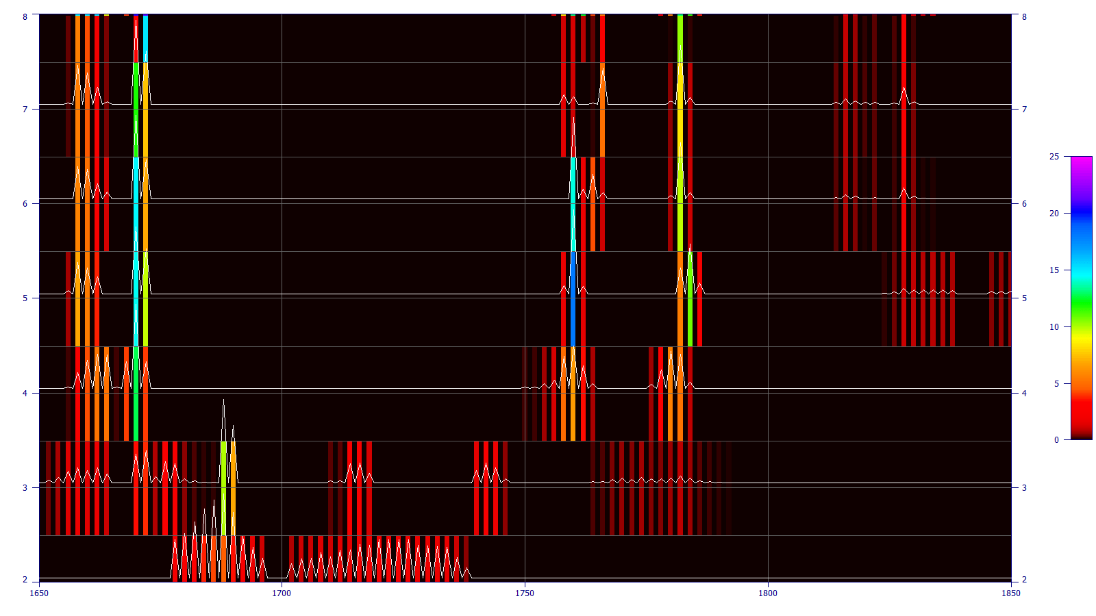
Confirmation of Pertinent Wavelengths
In direct spectral fits, far better estimates of significant wavelengths are realized. These tend to be much less influenced by secondary and inverse correlations or other artifacts arising from generating factor arrays. In the significance plot below, the contour reflects the weighted statistical significance for each wavelength that appears within the retained (best fit) models. At a certain parameter count and beyond, the significant wavelengths become sharply defined.
Modeling Technology and Code Export
From state-of-the-art outlier removal methods that allow you to refit and inspect a predictive model with the outliers removed, to writing the model code for you in C++ or Visual BASIC, PeakLab offers a full modeling solution from beginning to end. The C++ code below was generated from one of PeakLab’s sparse PLS models.
C++ Language Code – argument is specific spectra
double glm01(double *spec)
{
// spec[0] X Predictor 1 (1658, index=8)
// spec[1] X Predictor 2 (1660, index=10)
// spec[2] X Predictor 3 (1662, index=12)
// spec[3] X Predictor 4 (1664, index=14)
// spec[4] X Predictor 5 (1670, index=20)
// spec[5] X Predictor 6 (1672, index=22)
// spec[6] X Predictor 7 (1758, index=108)
// spec[7] X Predictor 8 (1760, index=110)
// spec[8] X Predictor 9 (1762, index=112)
// spec[9] X Predictor 10 (1766, index=116)
// spec[10] X Predictor 11 (1782, index=132)
// spec[11] X Predictor 12 (1816, index=166)
// spec[12] X Predictor 13 (1818, index=168)
// spec[13] X Predictor 14 (1822, index=172)
// spec[14] X Predictor 15 (1828, index=178)
double p[16]= {
4.06405812524123, -198.551348386628, -177.594084516741, -141.842381803743, -59.6348303087346,
280.22152394363, 538.494036162069, -216.618929884493, -759.483492213287, 778.463631058768,
-830.474230583933, 852.825799066597, 244.969804203827, 173.817451045103, 148.18538374493,
-630.888207432142,
};
int nx = 15;
double estimate = p[0];
for(int i=1; i<=nx; i++)
estimate += p[i]*spec[i-1];
return estimate;
}
A More Accurate and Far Simpler Alternative to PLS and PCR Models
The best direct spectral models should theoretically outperform optimum PLS and PCR models. For example, in PLS, some measure of the correlation latent variables will consist of random noise correlations and relationships with non-target components, moisture, or solvents. Experienced predictive modelers know that such predictive relationships are suspect, unreliable, far from robust, and are wisely never incorporated in a predictive system since these can vanish unexpectedly in real-world systems without warning. In general, such correlations are poorly understood, if at all, and are often blindly included in PLS and PCR modeling.
We have never encountered an ‘easy’ modeling scenario where PLS and PCR optimum factor counts could match the parameter count in direct spectral models, or where the prediction performance was as good. Even a simple case where a component could be efficiently predicted from a single spectral wavelength will typically optimize at three or four PLS factors or PCR principal components. Further, since PLS and PCR models must generally be converted back to the original spectral domain from the factor variables, those models may involve hundreds of parameters to address what a simple one wavelength direct spectral model manages with a higher prediction accuracy. Here is a white paper for a simple modeling example.
Similarly, we have equally never encountered a ‘difficult’ modeling scenario where the PLS and PCR factor counts weren’t higher than the parameter counts in an optimum spectral model, nor have we seen a case where the PLS or PCR models outperformed the direct spectral fits with respect to prediction accuracy. Here is a white paper for a complex modeling example where reflectance spectroscopy is impacted by particle size, moisture, and a massive obfuscation of the target components by other ingredients in a natural product.
Sound Mathematical and Statistical Science
PeakLab’s direct spectral fits use a full permutation procedure that can fit as many as a hundred million candidate fits in less than a minute, and in this procedure far more accurately determine the wavelengths where the deterministic information resides. Since no derived or latent variables are used, nothing is hidden, and random chance correlations and inverse relationships will not dominate the predictions.
The PeakLab direct spectral modeling produces true multivariate linear models which have been used in predictive models for decades and which are the bread and butter GLM models found in every major statistical software product in existence. Unlike PLS and PCR where this factor generation is usually hidden and proprietary, and where different PLS and PCR software will not produce exactly the same results, the PeakLab models can be replicated to full precision in any professional statistical software’s GLM procedure.
In using PeakLab to generate your spectral models, you are using the most stable, sound, and robust mathematical and statistical science available, and with an efficiency and ease of coding that will allow you to create web servers, embedded system handheld spectrometers, with ease. As part of PeakLab’s suite of analytical tools, the software cost for this modeling capability is a fraction of the price of commercial statistical or unscrambling software that is often purchased for chemometric modeling.