
Mixture Spectral Analysis: A Researcher’s Complete Guide

Mixture spectral analysis is defined as the mathematical decomposition of a composite spectral signal into its constituent components, called endmembers, along with their fractional abundances. The standard industry term for this process is spectral mixture analysis (SMA), and both terms describe the same core operation. SMA decomposes mixed pixel spectra into endmembers and estimates fractional abundances using the Linear Mixture Model (LMM). This technique drives material identification in remote sensing, quantitative analysis in chemistry, and signal deconvolution in hyperspectral imaging. Understanding SMA at the model level is the prerequisite for applying any of its modern variants correctly.
What is mixture spectral analysis and the Linear Mixture Model?
The Linear Mixture Model is the mathematical backbone of spectral mixture analysis. It expresses the observed spectrum as a weighted sum of endmember spectra plus a residual error term: Robs = Σ αi Ri + ε. Here, Robs is the measured spectral radiance, αi is the fractional abundance of each endmember i, Ri is the reference spectrum for that endmember, and ε is the residual error capturing noise and model imperfection. Each fractional abundance represents the proportion of a given material contributing to the observed signal at that pixel or sample location.
The physical interpretation of this equation is direct. If a sensor pixel covers a surface with 60% vegetation and 40% bare soil, the measured spectrum is approximately 0.6 times the vegetation endmember spectrum plus 0.4 times the soil endmember spectrum. The residual ε captures everything the linear model cannot explain, including sensor noise, atmospheric scattering, and genuine non-linear mixing effects. Keeping ε small is the practical goal of any well-calibrated SMA workflow.
The LMM carries two core assumptions that researchers must internalize before applying it. First, the model assumes linear additivity, meaning photons interact with only one material before reaching the sensor. Second, fractional abundances must satisfy sum-to-one and non-negativity constraints to remain physically meaningful. Unmixing algorithms must incorporate sum-to-one and non-negativity constraints to produce valid abundance estimates. Violating either constraint produces abundance values that have no physical interpretation.
- Define endmembers. Select or extract reference spectra for each pure material expected in the mixture.
- Apply abundance constraints. Enforce αi ≥ 0 and Σ αi = 1 before solving.
- Solve for fractional abundances. Use least-squares or constrained optimization to minimize ε.
- Evaluate residual error. Inspect ε spatially and spectrally to detect model violations.
Pro Tip: Always verify that your endmember spectra are measured under conditions matching your target data. A mismatch in illumination geometry or sensor calibration inflates ε and degrades abundance accuracy before you even begin unmixing.
What are the main methods for spectral mixture analysis?
Modern unmixing approaches are classified into three families: geometrical, statistical, and sparse regression-based methods. Each family addresses a different aspect of the unmixing problem, and the right choice depends on data dimensionality, endmember availability, and noise level.

Geometrical methods assume that pure endmembers occupy the vertices of a simplex in spectral feature space. Algorithms like N-FINDR and the Pixel Purity Index search for the data points that define the largest volume simplex, treating those points as endmembers. These methods work well when the data contain at least some near-pure pixels, which is common in high-resolution hyperspectral imagery. They struggle when all pixels are heavily mixed or when spectral dimensionality is very high.
Statistical methods model the distribution of spectral data rather than its geometry. Bayesian approaches place prior distributions over fractional abundances and endmember spectra, then infer posteriors using Markov Chain Monte Carlo or variational inference. This family handles noise more gracefully than geometrical methods and naturally incorporates uncertainty quantification. The trade-off is computational cost, which scales poorly with the number of endmembers and spectral bands.
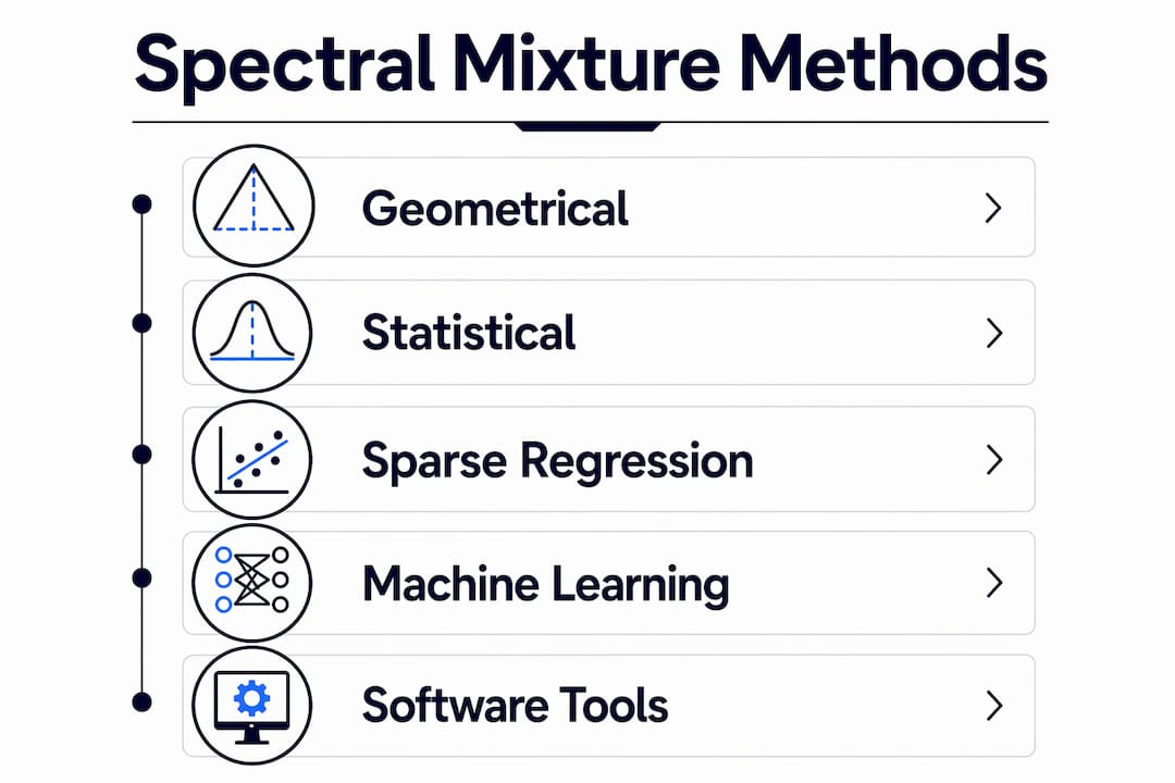
Sparse regression methods treat unmixing as a compressed sensing problem. A large spectral library serves as the dictionary, and the algorithm selects the smallest subset of library spectra that reconstructs the observed signal within a tolerance. This approach is powerful when a validated spectral library exists, as in mineral mapping or pharmaceutical analysis. For a detailed comparison of geometrical and statistical approaches, R2nsoftware provides a dedicated field guide covering method selection criteria.
| Method family | Core assumption | Typical use case | Key limitation |
|---|---|---|---|
| Geometrical | Pure pixels exist at simplex vertices | High-resolution hyperspectral imagery | Fails with fully mixed data |
| Statistical | Data follows a known distribution | Noisy or low-resolution data | High computational cost |
| Sparse regression | Observed spectra are sparse in a library | Mineral or pharmaceutical mapping | Requires a validated spectral library |
- Geometrical methods are fast and interpretable but require near-pure pixels.
- Statistical methods quantify uncertainty but demand significant computational resources.
- Sparse regression scales to large libraries but degrades when the library is incomplete.
Pro Tip: For sparse regression spectral unmixing, always validate your spectral library against independent field measurements before running the inversion. An outdated or incomplete library introduces systematic bias that no algorithm can correct.
What challenges make spectral mixture analysis difficult?
The mixed pixel problem is the most pervasive challenge in spectral mixture analysis. A single sensor pixel often covers multiple materials simultaneously, especially at coarse spatial resolutions. SMA applied to Sentinel-2 imagery of Tibet successfully separated mineral alteration signals from interfering vegetation, shadow, and water endmembers. That result required careful endmember selection and iterative residual analysis, not a single-pass inversion.
The unmixing problem is also fundamentally ill-posed. Multiple spectra can produce the same observed signal, meaning the solution is not unique without additional constraints. Researchers must impose physical priors, such as the sum-to-one condition, or regularization terms to select a single, meaningful solution from the infinite set of mathematically valid ones.
Endmember variability compounds this difficulty. Fixed reference spectra lead to inaccurate abundance estimates when environmental factors, grain size, or illumination angles shift the true endmember spectrum away from the library value. Dynamic or context-sensitive reference spectra address this, but they require more complex algorithms and larger calibration datasets.
“Unmixing is fundamentally an inverse problem requiring a careful choice of physical mixing models and quality endmember libraries for accurate results. Without these, even the most sophisticated algorithm returns physically meaningless abundance maps.”
- Noise sensitivity. Sensor noise propagates through the inversion, amplifying errors in low-abundance components.
- Non-linearity. Intimate mixtures, where photons scatter between particles of different materials, violate the LMM and require non-linear models.
- Dimensionality. High spectral dimensionality increases computation time and the risk of overfitting.
- Library completeness. Missing endmembers force residual error into the abundances of present endmembers, biasing all estimates.
Manual separation of spectral components is error-prone. Professional software tools that integrate baseline correction, noise filtering, and deconvolution reduce these errors systematically. For researchers dealing with overlapping spectral signals, automated deconvolution workflows provide a reproducible alternative to manual peak separation.
How are machine learning techniques advancing spectral mixture analysis?
Machine learning is reshaping mixture spectral methods at two distinct levels: the kernel level and the architectural level. Spectral mixture kernels in Gaussian Processes provide flexible, adaptive modeling of stationary kernels by combining Gaussian and Cauchy components to approximate complex spectral densities. This approach accelerates scientific discovery in fields like catalysis, where the spectral response of a catalyst surface changes continuously with reaction conditions. Static kernels cannot capture that variability; spectral mixture kernels can.
At the architectural level, the Mixture-of-Experts (MoE) framework integrates with spectral graph neural networks to improve modeling of graph-structured spectral data. The MoE framework treats eigengraph components as experts with learnable gating functions, improving both interpretability and scalability. Each expert specializes in a different frequency range of the graph spectrum, and the gating function dynamically weights their contributions based on the input. This mirrors the physical intuition of SMA, where each endmember contributes proportionally to the observed signal.
The practical benefits of these advances include:
- Adaptive modeling. Spectral mixture kernels adjust to multi-scale spectral features without manual kernel engineering.
- Scalability. MoE architectures distribute computation across experts, handling large hyperspectral datasets more efficiently than monolithic models.
- Interpretability. Learnable gating functions reveal which spectral components dominate in different spatial or chemical contexts.
- Improved inference. Spectral mixture kernels offer superior flexibility over static kernels, enabling multi-scale modeling for improved learning and inference.
Pro Tip: When applying Gaussian Process models with spectral mixture kernels to analytical chemistry data, initialize kernel hyperparameters using the power spectral density of your training data. Random initialization in high-dimensional spectral spaces frequently converges to local optima that underfit the dominant frequency components.
What are practical applications and examples of mixture spectral analysis?
Spectral mixture analysis techniques appear across a wide range of scientific and industrial contexts. The following examples illustrate how the methods described above translate into measurable analytical outcomes.
-
Mineral mapping from satellite imagery. Hyperspectral sensors like AVIRIS or Sentinel-2 collect hundreds of spectral bands per pixel. SMA separates mineral endmembers such as kaolinite, alunite, and iron oxides from vegetation and shadow contributions, producing fractional abundance maps that guide geological surveys.
-
Environmental monitoring. Water quality analysts use SMA to decompose the reflectance spectrum of a water body into contributions from phytoplankton, suspended sediment, and dissolved organic matter. Each component has a distinct spectral signature, and fractional abundances correlate with concentration.
-
FT-IR analysis of chemical mixtures. Advanced spectral unmixing workflows integrate baseline correction, noise filtering, and deconvolution to manage non-linear and overlapping spectral phenomena. In pharmaceutical quality control, FT-IR SMA quantifies active ingredient concentrations in tablet formulations without physical separation.
-
Hyperspectral medical imaging. Tissue samples imaged with hyperspectral cameras yield mixed spectra from collagen, hemoglobin, and lipid components. SMA decomposes these signals to map tissue composition at the pixel level, supporting histological analysis.
-
Chromatographic peak deconvolution. In chromatography, co-eluting compounds produce overlapping detector signals. Spectral mixture methods applied to diode-array or mass spectrometry data resolve individual component spectra and quantify their contributions, recovering accuracy that single-wavelength detection cannot achieve.
Key Takeaways
Spectral mixture analysis requires a validated Linear Mixture Model, physically constrained abundance estimation, and method selection matched to data geometry, noise level, and endmember availability.
| Point | Details |
|---|---|
| LMM is the foundation | Every SMA workflow begins with R_obs = Σ αi R_i + ε; constraints on αi are non-negotiable. |
| Method choice matters | Geometrical, statistical, and sparse regression methods each suit different data conditions. |
| Endmember variability is a primary error source | Dynamic reference spectra reduce bias when environmental or physical conditions shift endmember signatures. |
| Machine learning extends SMA | Spectral mixture kernels and MoE architectures improve adaptability and scalability beyond classical LMM. |
| Software quality determines reproducibility | Automated baseline correction and deconvolution reduce manual error and produce defensible results. |
Why the foundations of SMA still matter more than the algorithms
Researchers entering the field often focus on algorithm selection before they have a firm grip on the LMM and its constraints. That ordering is backward. Every advanced method, whether a Gaussian Process with spectral mixture kernels or an MoE graph network, still depends on the quality of the endmember library and the physical validity of the abundance constraints. A sophisticated algorithm applied to a poorly curated endmember set produces confident-looking but wrong results.
The challenge I see most often in practice is not computational. It is the assumption that more spectral bands or a larger training set will compensate for weak domain knowledge. They do not. Endmember variability caused by grain size or illumination angle shifts the reference spectrum in ways that no amount of data augmentation corrects without explicit physical modeling. The researchers who get reliable results are the ones who invest time in field validation and library curation before they run a single inversion.
Machine learning integration is genuinely useful, but it works best as an extension of classical SMA, not a replacement. Spectral mixture kernels accelerate Bayesian optimization in catalysis because they encode the right inductive bias for spectral data. They do not eliminate the need to understand what the spectral density of your data actually represents. My advice to students and researchers: master the LMM, understand why the sum-to-one constraint exists physically, and then layer on the advanced methods. The sequence matters.
— Nadeem
R2nsoftware tools for spectral data deconvolution
Researchers who need to move from SMA theory to reproducible analytical results will find that software architecture matters as much as method selection.

R2nsoftware’s PeakLab supports up to 1,000 peaks simultaneously, resolving overlapping signals that classical single-pass methods cannot separate. Its integrated baseline correction and noise filtering align directly with the workflow requirements described throughout this article. For signal-level deconvolution and automated spectral unmixing, AutoSingal provides algorithm-driven separation of composite spectral signals with reproducible, statistically defensible outputs. R2nsoftware also maintains a library of tutorial videos covering practical SMA workflows, from endmember selection through abundance mapping and residual analysis.
FAQ
What is spectral mixture analysis in simple terms?
Spectral mixture analysis is the process of mathematically separating a combined spectral signal into the individual spectra of its component materials and estimating how much each material contributes to the observed signal.
How does the Linear Mixture Model work?
The LMM expresses the observed spectrum as a weighted sum of endmember spectra, where the weights are fractional abundances constrained to be non-negative and sum to one, plus a residual error term.
What are the main mixture spectral analysis techniques?
The three main families are geometrical methods, which locate endmembers at simplex vertices; statistical methods, which model data distributions; and sparse regression methods, which select endmembers from a spectral library.
Why is endmember variability a problem in SMA?
Environmental factors, grain size, and illumination angles shift the true endmember spectrum away from the fixed library value, causing the model to misattribute spectral contributions and produce biased abundance estimates.
Where is mixture spectral analysis used in chemistry?
SMA is applied in FT-IR analysis of pharmaceutical formulations, hyperspectral tissue imaging, chromatographic peak deconvolution, and environmental water quality monitoring to quantify component concentrations without physical separation.