Statistical Models for Spectral Data: A Researcher’s Guide

Statistical modeling for spectral data is defined as the application of mathematical frameworks, including regression, nonlinear, and generative methods, to extract quantitative and qualitative chemical or physical information from measured spectra. The types of statistical models for spectral data span a broad spectrum, from foundational partial least squares (PLS) regression to generative adversarial networks (GANs), each addressing distinct analytical challenges. Researchers working in spectroscopy, chromatography, and hyperspectral imaging rely on these models to resolve overlapping peaks, separate signal from noise, and produce reproducible, scientifically defensible results. Selecting the right model class directly determines the accuracy of peak identification and the fidelity of signal resolution.

1. What are the types of statistical models for spectral data?

Statistical models applied to spectral analysis fall into three broad categories: linear regression models, nonlinear models, and generative models. Each category addresses a different level of data complexity. Linear models work well when spectral responses scale proportionally with analyte concentration. Nonlinear and generative models become necessary when instrument artifacts, overlapping bands, or matrix effects introduce complexity that linear assumptions cannot capture.

Data-driven approaches enable consistent parameter extraction across large spectral surveys, even at low resolution or low signal-to-noise ratios. This means no single model class dominates all scenarios. The choice depends on data dimensionality, noise characteristics, and whether interpretability or predictive accuracy takes priority.

2. Regression-based models: the foundation of spectral analysis

Partial least squares regression and ordinary least squares (OLS) regression are the foundational linear models in spectral data analysis. PLS handles the high collinearity typical of spectral data by projecting both predictors and responses into a lower-dimensional latent space. OLS works when the number of spectral variables is smaller than the number of samples and multicollinearity is not a concern.

Key linear regression approaches for spectral data include:

• PLS regression: Reduces dimensionality while preserving covariance between spectral predictors and analyte concentrations.
• OLS regression: Applies when spectral features are pre-selected and the design matrix is well-conditioned.
• Polynomial regression: Captures mild nonlinearities by adding squared or cubic spectral terms to the model.
• Inverse least squares (ILS): Regresses concentration directly on spectral intensities, useful when the number of calibration samples is large.

Complex-valued ILS applied to absorbance or Raman spectra can match or outperform conventional PLS by pairing measured intensities with Kramers–Kronig derived real parts. This finding challenges the assumption that PLS is always the default best choice for spectral regression. Researchers working with Raman or infrared data should evaluate complex-valued formulations before defaulting to standard real-valued PLS.

Pro Tip: When building a PLS calibration model, always validate with an independent external test set rather than relying solely on cross-validation statistics. Cross-validation can mask overfitting when spectral variables are highly correlated.

The primary limitation of linear regression models is their inability to capture strong nonlinear relationships between spectral features and analyte properties. When spectral responses exhibit saturation, peak shifts, or matrix-dependent band broadening, polynomial extensions or kernel methods become necessary.

3. How advanced nonlinear models enhance spectral data analysis

Nonlinear spectral data modeling techniques address the limitations of linear regression when spectral responses are governed by complex physical or chemical interactions. Nonlinear modeling methods include polynomial regression, kernel partial least squares (K-PLS), Gaussian process regression (GPR), and artificial neural networks (ANNs), each suited to different levels of data complexity.

The four primary nonlinear model types for spectral analysis are:

• Kernel PLS (K-PLS): Maps spectral data into a high-dimensional feature space using kernel functions, capturing nonlinear concentration-spectral relationships without explicitly computing the transformation.
• Gaussian process regression (GPR): Provides a fully probabilistic model with built-in uncertainty quantification. GPR is preferred when confidence intervals on predictions are scientifically required.
• Artificial neural networks (ANNs): Handle large-scale, high-dimensional spectral datasets with complex nonlinear mappings. ANNs handle complex nonlinear mappings but may overfit with limited calibration samples and challenge interpretability for scientific insight.
• Support vector regression (SVR): Maximizes the margin between predicted and actual values, performing well on moderate-sized spectral datasets with clear nonlinear structure.

Gaussian process regression is preferred when uncertainty quantification is critical, while ANNs excel at large-scale nonlinear problems. This trade-off is not merely academic. In pharmaceutical spectroscopy, where regulatory submissions require prediction uncertainty estimates, GPR provides a statistically rigorous framework that ANNs cannot easily replicate without additional calibration steps.

Computational cost is the primary constraint on GPR adoption. Scaling GPR to hyperspectral imaging datasets with thousands of spectral channels requires sparse approximations or inducing-point methods. ANNs scale more readily but demand large, well-curated training sets to avoid overfitting.

4. What role do generative AI models play in spectral data modeling?

Generative models represent a fundamentally different class of spectral data modeling techniques. Where predictive models map spectra to analyte properties, generative models learn the underlying distribution of spectral data itself. This distinction matters because generative models can simulate realistic spectra, augment calibration sets, and quantify uncertainty in ways that discriminative models cannot.

Core generative approaches for spectral analysis include:

• Variational autoencoders (VAEs): Encode spectral data into a compressed latent representation and decode it back, learning the statistical structure of spectral shapes, noise, and physical variability.
• Generative adversarial networks (GANs): Train a generator and discriminator in competition, producing synthetic spectra that are statistically indistinguishable from measured data.
• Diffusion models: Reconstruct spectral signals by learning to reverse a noise-addition process, enabling high-fidelity spectral simulation even under low signal-to-noise conditions.

Generative models learn spectral shapes, correlations, noise, and physical variability, offering modern chemometric extensions beyond traditional methods. This positions generative AI not as a replacement for classical chemometrics but as an extension that addresses calibration gaps and data scarcity.

Pro Tip: Use VAE-generated synthetic spectra to augment calibration sets when physical sample preparation is constrained by cost or material availability. Validate synthetic spectra against measured reference standards before including them in production calibration models.

The practical benefit of generative models is most pronounced in scenarios where collecting large calibration sets is impractical. Pharmaceutical process analytical technology (PAT) applications, for example, often require calibration across a wide range of process conditions that cannot all be physically sampled. GANs and VAEs fill this gap by generating spectra that represent unsampled process states.

5. How automated frameworks optimize model selection for spectral data

Manual model selection across the full space of regression algorithms, feature subsets, and hyperparameters is not tractable for most spectral analysis workflows. The number of possible model configurations grows combinatorially with spectral dimensionality. Automated frameworks address this by applying Bayesian optimization and high-throughput computing to identify optimal configurations efficiently.

The AutoRegress framework uses parallelized Bayesian optimization and strict cross-validation to identify optimal regression models and feature subsets in spectral data. Automated Bayesian optimization over 2,800 models achieved an external test R² of 0.9722 and an RMSE of 0.2256. That level of predictive accuracy, achieved without manual model tuning, demonstrates that automation does not sacrifice performance for convenience.

The workflow of an automated spectral modeling framework follows a structured sequence:

1. Feature pre-selection: Spectral regions are filtered using variance thresholds or correlation-based criteria to reduce the initial feature space.
2. Model candidate generation: Regression algorithms including PLS, SVR, GPR, and ANN variants are instantiated across a defined hyperparameter grid.
3. Bayesian optimization: A surrogate model predicts which configurations are most likely to improve validation performance, directing computational resources efficiently.
4. Cross-validation: Each candidate model is evaluated using k-fold or leave-one-out cross-validation to prevent overfitting.
5. External test evaluation: The top-ranked model is applied to a held-out external test set to confirm generalization.

Automated frameworks reduce human bias and time investment in spectral data analysis workflows. This is particularly significant in multi-site studies where analyst-to-analyst variability in model selection can introduce systematic differences in reported results. Automation enforces a consistent, reproducible selection protocol across all sites.

Researchers can explore the regression analysis workflow developed by R2nsoftware for a structured approach to applying automated model selection in spectroscopy contexts.

6. What factors influence model choice for different spectral scenarios?

The best statistical methods for spectra depend on four intersecting factors: dataset size, spectral dimensionality, noise level, and the required balance between interpretability and predictive accuracy. No single model class is universally optimal. Selecting the wrong model for a given spectral scenario produces systematic prediction errors that propagate through downstream chemical conclusions.

Factors governing model selection in spectral analysis include:

• Dataset size: PLS and OLS perform reliably with small calibration sets (fewer than 100 samples). ANNs and GPR require substantially larger datasets to avoid overfitting.
• Spectral dimensionality: High-dimensional hyperspectral data (thousands of channels) favors dimensionality-reducing methods like PLS or K-PLS before applying nonlinear layers.
• Noise level: Data-driven models provide consistent parameter estimation even at low signal-to-noise ratios, making them preferable over purely theoretical models in noisy instrument environments.
• Interpretability requirements: Regulatory submissions in pharmaceutical or food safety contexts often require interpretable models. PLS loadings and regression coefficients are auditable. ANN weights are not.
• Nonlinearity severity: Mild nonlinearity warrants polynomial extensions of PLS. Severe nonlinearity from matrix effects or overlapping band systems warrants K-PLS or ANN approaches.

Emerging hybrid models combine theoretical spectral line shapes, such as Voigt or Lorentzian profiles, with data-driven residual correction layers. This approach preserves physical interpretability while allowing the data-driven component to absorb unexplained variance. For researchers working on complex mixture analysis, hybrid models represent the most defensible path when both accuracy and interpretability are required.

The practical guidance is direct: start with PLS as the baseline, test polynomial and kernel extensions if residuals show systematic nonlinear patterns, and reserve ANNs or generative models for scenarios where dataset size and computational resources support their demands.

Key Takeaways

The most effective approach to statistical modeling for spectral data is to match model complexity to data characteristics, starting with interpretable linear models and escalating to nonlinear or generative methods only when residual analysis confirms their necessity.

Point	Details
PLS as the baseline	Partial least squares handles collinearity and dimensionality in most spectral calibration scenarios.
Nonlinear escalation path	Move from polynomial regression to K-PLS or GPR when residuals show systematic nonlinear patterns.
Generative models for data scarcity	VAEs and GANs augment calibration sets when physical sample collection is constrained.
Automation reduces bias	Bayesian-optimized frameworks evaluate thousands of configurations, achieving R² above 0.97 without manual tuning.
Interpretability governs regulatory use	Regulatory submissions require auditable models; PLS loadings satisfy this requirement where ANN weights do not.

What I’ve learned about model selection in spectral analysis

After working extensively with spectral datasets across chromatography and spectroscopy applications, the most persistent mistake I observe is treating PLS as a universal solution rather than a starting point. PLS is excellent, but it is a linear model applied to data that is frequently nonlinear. Analysts who skip residual analysis after fitting PLS miss systematic errors that compound across the calibration range.

The rise of automated frameworks like AutoRegress has genuinely changed the practical workflow. I used to spend days manually testing model configurations. Bayesian-optimized automation compresses that process into hours and removes the subjective element from model selection. The reproducibility gains alone justify the adoption.

Generative models are the area I watch most closely. The ability to simulate physically realistic spectra for process conditions that cannot be sampled directly solves a calibration problem that has constrained PAT applications for years. The key discipline is validation: synthetic spectra must be benchmarked against measured reference standards before entering any production model.

My strongest advice is to invest in understanding your spectral data’s noise structure before selecting any model. Noise that is heteroscedastic, instrument-dependent, or correlated across spectral channels changes which model class will generalize. Domain knowledge about the instrument response function is not optional. It is the foundation on which every statistical model either succeeds or fails.

— Nadeem

R2nsoftware tools for automated spectral modeling

R2nsoftware provides analytical tools built specifically for the demands of spectral peak identification, signal resolution, and regression modeling in research environments.

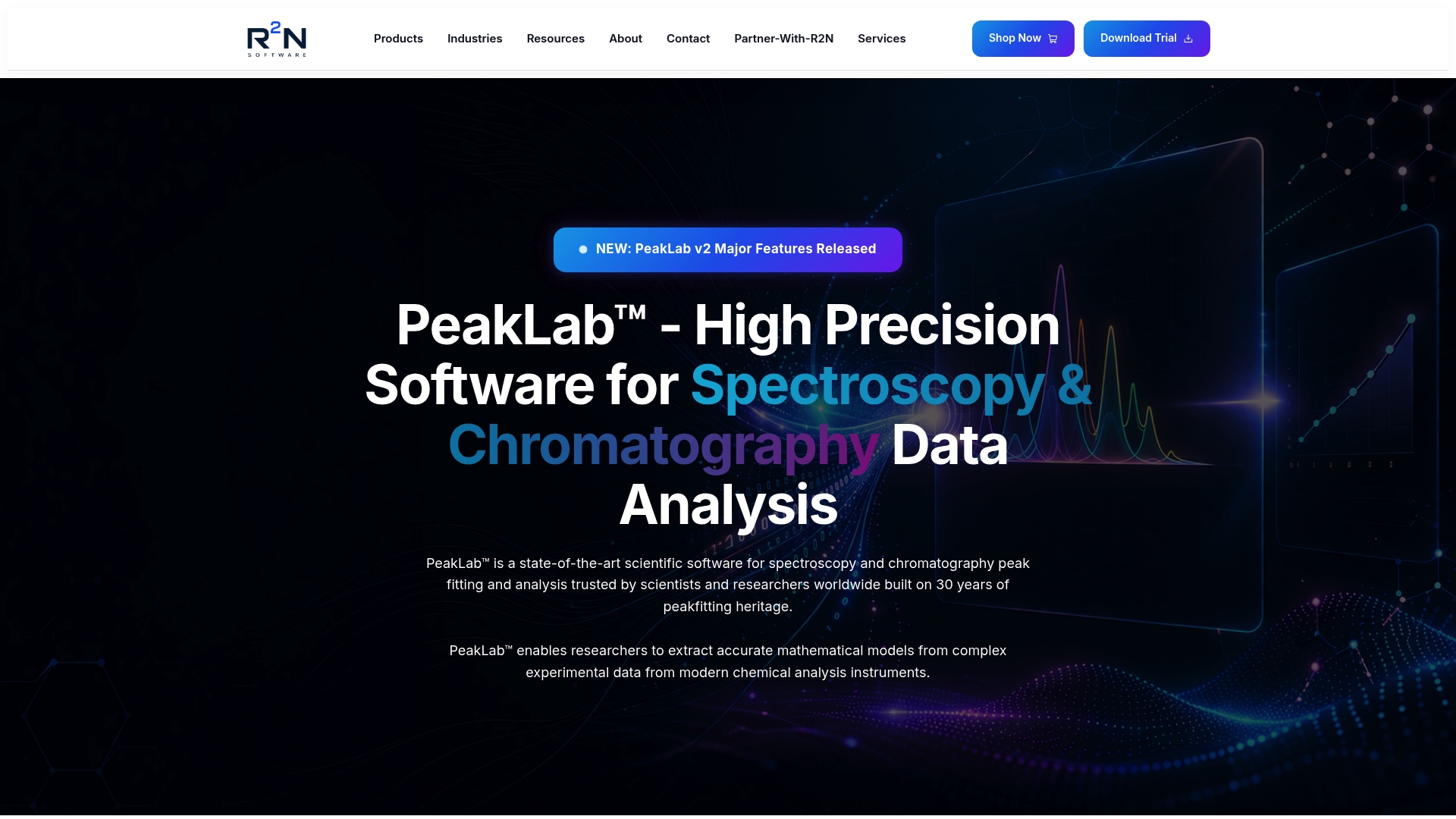
AutoSingal delivers automated signal detection and regression modeling for spectral data, applying the same class of optimization logic discussed throughout this article. PeakLab™ supports up to 1,000 simultaneous peaks, resolving overlapping signals that standard regression tools cannot separate. Researchers who need to move from raw spectral data to defensible quantitative results without manual model tuning will find both tools directly applicable. The PeakLab platform also integrates baseline correction and curve fitting within a single workflow, reducing the number of software transitions required during analysis.

FAQ

What is the most widely used statistical model for spectral data?

Partial least squares (PLS) regression is the most widely used model in spectral analysis. It handles high collinearity and dimensionality reduction simultaneously, making it the standard baseline for calibration in spectroscopy and chromatography.

When should researchers use nonlinear models instead of PLS?

Nonlinear models are appropriate when residual analysis after PLS fitting reveals systematic, concentration-dependent errors. Kernel PLS, Gaussian process regression, and ANNs each address different scales of nonlinearity depending on dataset size and interpretability requirements.

How do generative AI models improve spectral calibration?

Generative models such as VAEs and GANs simulate realistic spectra by learning the statistical distribution of measured data, including noise and physical variability. They augment calibration sets in scenarios where collecting sufficient physical samples is impractical.

What is the benefit of automated model selection for spectral analysis?

Automated frameworks using Bayesian optimization evaluate thousands of model and feature configurations with minimal user input, achieving high predictive accuracy while removing analyst bias from the selection process.

Can complex-valued regression outperform standard PLS for spectral data?

Complex-valued ILS applied to absorbance or Raman spectra reduces prediction errors compared to conventional real-valued PLS in specific scenarios, suggesting that the standard regression hierarchy should be re-evaluated when complex spectral representations are available.

Recommended

• Blog – R2N Software
• Statistical Modeling for Complex Mixtures: A Field Guide – R2N Software
• Regression Analysis Spectroscopy Data Workflow Guide – R2N Software
• The Role of Statistical Models in Data Analysis – R2N Software