
Voigt Function for Defensible Peak Fitting
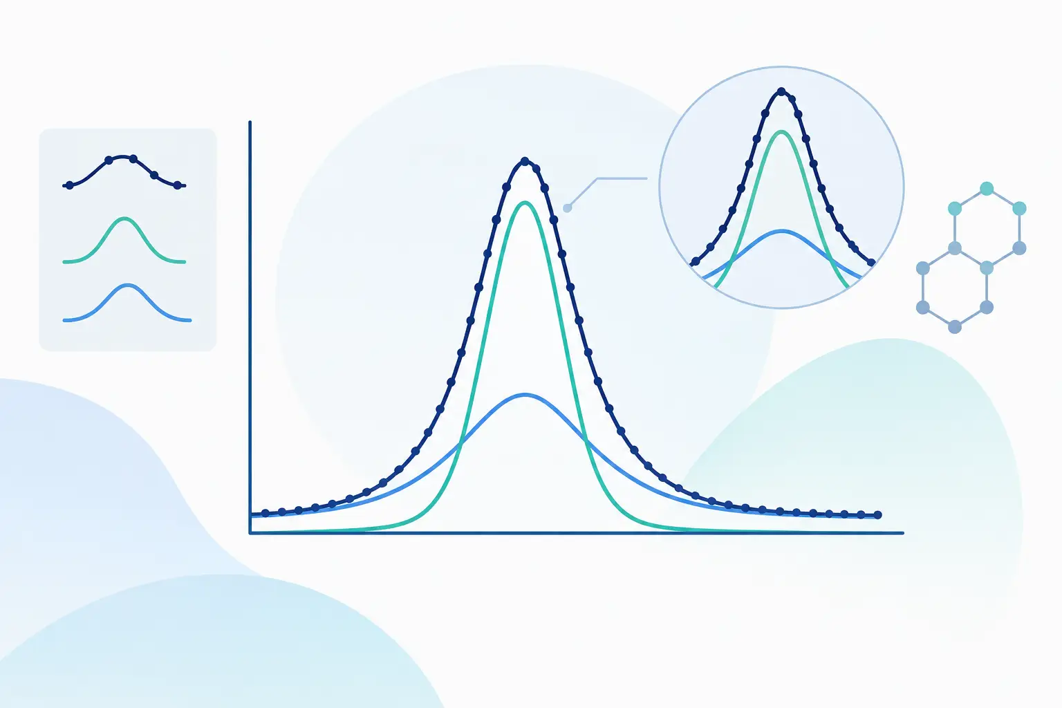
A peak that appears symmetric is not necessarily Gaussian, and a good-looking fit is not necessarily a valid analytical model. The voigt function is often the appropriate choice when measured line shapes reflect more than one physical broadening mechanism. It combines Gaussian and Lorentzian behavior in a single peak profile, allowing scientists to model real instrumental and sample-driven effects without forcing complex data into an oversimplified shape.
For spectroscopy, chromatography, mass spectrometry, and materials characterization, that distinction affects more than residual error. Peak position, area, width, resolution, and uncertainty estimates all depend on whether the chosen line shape represents the observed signal. When overlapping peaks are present, a poorly selected profile can redistribute area between components, shift centroids, and produce conclusions that cannot be defended in a publication, technical review, or regulated workflow.
What the Voigt Function Represents
The Voigt profile is the convolution of a Gaussian function and a Lorentzian function. In practical terms, it describes a peak shaped by two broadening contributions acting together rather than independently competing for the same data.
A Gaussian component commonly represents effects that arise from many small, statistically distributed variations. Instrumental resolution, Doppler broadening, detector response, and certain population-level variations can produce approximately Gaussian broadening. Its tails decline relatively quickly as distance from the peak center increases.
A Lorentzian component is associated with mechanisms that produce broader tails. Natural lifetime broadening, collision-related effects, relaxation processes, and some resonance phenomena can contribute Lorentzian behavior. A Lorentzian peak may look similar to a Gaussian near its apex, yet its slower-decaying tails can materially alter the fit in regions that appear visually unimportant.
Mathematically, the Voigt profile is written as the convolution:
`V(x; sigma, gamma) = integral from -infinity to infinity of G(x’; sigma) L(x – x’; gamma) dx’`
Here, `sigma` is the Gaussian standard deviation and `gamma` is the Lorentzian half-width at half-maximum. These parameters should not be confused with interchangeable width controls. The Gaussian full width at half maximum is `2.35482 sigma`, while the Lorentzian full width at half maximum is `2 gamma`. Reporting the wrong width definition is a common source of avoidable ambiguity when comparing fitted peaks across methods or laboratories.
Why a Voigt Function Can Change the Interpretation
A Gaussian-only model can underestimate the tails of a broadened line. A Lorentzian-only model can overemphasize them and distort the central region. Either error may be modest for an isolated, high signal-to-noise peak. It becomes much more consequential when components overlap, a baseline is structured, or a weak peak lies on the shoulder of a stronger one.
Consider two partially resolved spectral bands. If the actual bands have Voigt-like tails but are fitted as Gaussians, the fitting routine may compensate by widening one component, shifting centers, or introducing an extra peak. The final graph may look acceptable, but the component areas and derived concentrations can be biased. Conversely, applying Lorentzian shapes to predominantly Gaussian peaks may create artificial tail contributions that absorb baseline curvature or noise.
This is why line-shape selection is a modeling decision, not a cosmetic setting. The correct question is not, “Which curve follows the trace?” It is, “Which model explains the trace with physically plausible parameters, statistically acceptable residuals, and the fewest unsupported assumptions?”
When the Voigt Function Is the Right Peak Model
The Voigt function is especially useful when independent evidence suggests that both Gaussian and Lorentzian broadening are active. It is widely applicable to absorption and emission spectroscopy, Raman and infrared analysis, X-ray photoelectron spectroscopy, diffraction, NMR, and certain mass-spectrometric or chromatographic signals where peak tails cannot be represented adequately by a purely Gaussian profile.
There is no universal rule that every peak should be Voigt. In chromatography, for example, asymmetry from column interactions, overload, gradient effects, or detector dynamics may require an asymmetric peak model rather than a symmetric Voigt profile. In mass spectra, isotopic patterns, detector saturation, and unresolved ion populations can demand domain-specific constraints that a single generic line shape cannot supply.
The model choice also depends on data quality. A Voigt fit has more flexibility than a pure Gaussian or Lorentzian fit. If the signal contains few points across the peak, has low signal-to-noise ratio, or includes severe baseline uncertainty, the Gaussian and Lorentzian contributions may not be independently identifiable. More parameters do not automatically produce more knowledge.
Fit the Baseline and Peaks as One Analytical Problem
Peak fitting fails most often before the optimizer reaches the peak parameters. A baseline that is manually subtracted, poorly estimated, or treated as fixed can force the peak model to absorb drift and curvature. That affects width, area, and the apparent Lorentzian tail contribution.
A defensible workflow models baseline and peak behavior together. The baseline should be sufficiently flexible to represent known background structure, but constrained enough that it does not consume genuine low-intensity peaks or broad spectral features. The peak model should then be fit over a region that includes enough of each peak’s shoulders and tails to distinguish line shape from background.
Parameter bounds and scientific constraints are equally important. Centers may be restricted to known transition positions or retention windows. Widths can be constrained to physically reasonable ranges. Peak areas may be required to remain positive. In multipeak models, known spacing, shared widths, isotopic ratios, or theoretical area relationships can reduce parameter correlation and make a complex fit identifiable.
These decisions must be traceable. A reproducible analysis records the baseline model, line-shape choice, parameter limits, initial conditions, fitting range, weighting strategy, convergence criteria, and uncertainty calculation. Without that record, a fitted curve is difficult to reproduce even when the raw data are available.
Evaluate More Than the Residual Sum of Squares
A lower residual sum of squares does not prove that a Voigt model is correct. It only indicates that the selected model has reduced the difference between observed and calculated values. A flexible model can fit noise, baseline artifacts, or unmodeled interference if it is not challenged by diagnostic evidence.
Residual plots provide the first check. Random residuals distributed around zero are more credible than residuals with a repeating structure, broad wings, center-region bias, or a systematic sign change near overlapping peaks. Residual autocorrelation can reveal that apparent improvements in fit quality are merely tracking correlated noise or baseline structure.
Model comparison criteria such as adjusted R-squared, Akaike information criterion, Bayesian information criterion, and parameter confidence intervals add useful perspective. A Voigt model may outperform a Gaussian model statistically, but the improvement must justify the added freedom. If the Lorentzian width is poorly determined, highly correlated with the Gaussian width, or driven to a parameter boundary, the dataset may not support a full Voigt interpretation.
The fitted parameters should also make scientific sense. A narrow Gaussian contribution paired with an implausibly broad Lorentzian term may point to unresolved components, an incomplete baseline model, detector artifacts, or an inappropriate fitting range. Statistical output and domain knowledge must agree before a result becomes actionable.
Voigt Function Versus Pseudo-Voigt Approximation
A pseudo-Voigt function is a weighted sum of Gaussian and Lorentzian profiles rather than their true convolution. It is computationally convenient and can approximate a Voigt shape closely in many applications. For high-throughput screening, initial parameter estimation, or datasets where the distinction is below experimental precision, a pseudo-Voigt model may be entirely appropriate.
The trade-off is interpretability and accuracy. The mixing fraction in a pseudo-Voigt model is not always equivalent to a direct physical partition of Gaussian and Lorentzian broadening. When line-shape parameters are central to the scientific interpretation, or when highly overlapped peaks require small differences in tail behavior to be resolved, the true Voigt function is generally the more defensible choice.
Modern numerical implementations make true Voigt evaluation practical for routine nonlinear fitting. The remaining challenge is not calculation speed alone. It is setting up the full model correctly, including baseline terms, component count, constraints, weighting, and diagnostic review. Specialized environments such as PeakLab are designed around that complete analytical workflow rather than treating peak shape as an isolated curve-fitting option.
Turning a Voigt Fit Into a Defensible Result
A Voigt fit earns confidence when it survives comparison. Fit the same region using scientifically plausible alternatives, inspect the residual structure, examine parameter correlations, and test whether conclusions such as peak area ratios or component positions remain stable. If small changes in starting values or baseline settings produce large changes in the result, the model is not yet sufficiently constrained.
For reporting, state the profile definition and width convention explicitly. Identify whether the model is a true Voigt or pseudo-Voigt, describe baseline handling, report uncertainty estimates, and retain the fitting configuration with the raw data. These details convert a visually persuasive curve into a result another scientist can reproduce and evaluate.
The value of the Voigt function is not that it makes every peak fit better. Its value is that, when the data and underlying physics warrant it, it gives broadening mechanisms, overlap behavior, and fitted parameters a more credible analytical foundation.