
Statistical Modeling Science: A Guide for Researchers

Statistical modeling science is the mathematical and probabilistic framework for representing relationships between variables in observed data, using explicitly encoded assumptions to support inference, prediction, and decision-making. Known formally as statistical modeling, this discipline sits at the core of quantitative research across fields from epidemiology to spectroscopy. A statistical model is a mathematical representation of the data-generating process, relating random to fixed variables under explicit assumptions. Every statistical hypothesis test and estimator derives from a statistical model, which means the discipline is not a peripheral tool but the foundation of statistical inference itself. Researchers who understand what is statistical modeling science gain the ability to translate domain questions into testable, quantifiable frameworks.
What is statistical modeling science and its core components?
Statistical modeling science is the practice of specifying mathematical relationships between variables, encoding probability distributions, and estimating unknown parameters from data. A statistical model embodies a set of statistical assumptions concerning the generation of sample data and probability distributions parameterized by unknown parameters. That definition has a direct consequence: every modeling decision, from choosing a distribution to specifying which variables interact, encodes a scientific assumption about reality.
The building blocks of any statistical model fall into two categories: deterministic elements and stochastic elements. Deterministic elements describe the fixed, systematic part of a relationship, such as a linear trend between dose and response. Stochastic elements capture random variation, the noise that real data always contain. Even for phenomena that are theoretically deterministic, stochastic assumptions accommodate noise and enable valid inference from imperfect measurements.

Variables in a model are classified as either random or non-random. Non-random variables, often called covariates or predictors, are treated as fixed and known. Random variables carry probability distributions and represent outcomes or errors. Parameters are the numerical quantities that define those distributions, and parameterization is the process of specifying which parameters the model will estimate from data.
Common model types include:
- Regression models: Estimate a continuous outcome as a function of one or more predictors.
- Classification models: Assign observations to discrete categories using probability thresholds.
- Clustering models: Group observations by similarity without predefined labels.
- Time series models: Capture temporal dependence in sequentially ordered data.
Each type formalizes a different scientific hypothesis about how data are generated.
Pro Tip: Before selecting a model type, write down the scientific question in plain language. If the question asks “how much,” use regression. If it asks “which group,” use classification. Matching the model type to the question prevents the most common modeling errors.
How does maximum likelihood estimation quantify model parameters?
Maximum likelihood estimation (MLE) is the most widely used method for fitting parameters in statistical models. MLE selects parameter values that maximize the likelihood of the observed data under the assumed model. The intuition is direct: among all possible parameter configurations, MLE identifies the one that makes the observed data most probable.
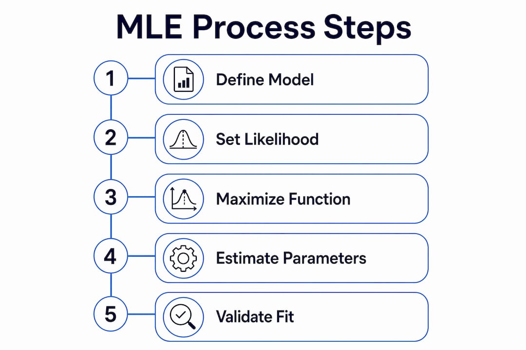
The likelihood function maps every point in the parameter space to a probability value for the observed data. Maximizing that function, typically by taking derivatives and solving for zero, yields the maximum likelihood estimates. In practice, researchers maximize the log-likelihood because logarithms convert products into sums, which are computationally simpler to handle.
MLE has well-established theoretical properties. Under regularity conditions, MLE estimates are consistent, meaning they converge to the true parameter values as sample size grows. They are also asymptotically efficient, achieving the lowest possible variance among unbiased estimators. These properties explain why MLE appears in linear regression, logistic regression, Poisson models, and survival analysis.
Alternative estimation approaches include:
- Bayesian estimation: Combines the likelihood with a prior distribution over parameters, producing a posterior distribution rather than a point estimate.
- Quasi-likelihood: Relaxes full distributional assumptions, requiring only a specification of the mean-variance relationship.
- Method of moments: Matches theoretical moments to sample moments, useful when the likelihood is intractable.
Each alternative trades off assumptions against computational cost or interpretability.
Pro Tip: When fitting regression coefficients, always inspect the log-likelihood surface for flatness or multiple peaks. A flat surface signals weak identifiability, meaning the data do not strongly constrain the parameter estimate regardless of sample size.
What principles guide model selection and evaluation?
Model selection is the process of choosing among competing candidate models based on criteria that balance fit against complexity. Model selection uses criteria such as the Akaike information criterion (AIC) and the Bayesian information criterion (BIC) to balance goodness of fit with parsimony. The underlying principle is Occam’s razor: the simplest model that adequately fits the data is preferred over a more complex one.
The table below compares the three most common selection criteria:
| Criterion | Penalizes complexity by | Best suited for |
|---|---|---|
| AIC | 2 × number of parameters | Predictive accuracy |
| BIC | log(n) × number of parameters | Inference and model identification |
| Bayes factor | Marginal likelihood ratio | Formal hypothesis comparison |
The distinction between selecting a model for inference versus prediction matters. For inference, you want a model whose parameters are interpretable and whose assumptions are defensible. For prediction, you prioritize out-of-sample accuracy, which may favor a model with more parameters if the training data are large. Model complexity and estimate stability are intertwined: adding parameters always improves in-sample fit but can destabilize estimates and reduce interpretability.
Identifiability is a prerequisite for valid model selection. A model is identifiable if different parameter values produce different probability distributions. Non-identifiable models cannot be estimated reliably regardless of sample size or criterion used. Researchers should verify identifiability analytically before fitting any model to data.
How do generalized linear models illustrate statistical modeling flexibility?
Generalized linear models (GLMs) are a unified family of statistical models that extend linear regression to accommodate non-normal outcome distributions. GLMs generalize linear regression by linking the mean outcome to predictors via a link function, with parameters estimated by maximum likelihood or Bayesian methods. The link function transforms the predicted mean so that it remains within a valid range for the outcome type.
The table below summarizes three core GLM variants:
| GLM type | Distribution | Link function | Typical use case |
|---|---|---|---|
| Linear regression | Gaussian | Identity | Continuous outcomes |
| Logistic regression | Binomial | Logit | Binary outcomes |
| Poisson regression | Poisson | Log | Count data |
Each row represents a different scientific context, yet all three share the same estimation framework and model selection logic. GLMs provide a unified modeling approach where various response variables are handled by adjusting distribution assumptions and link functions. That unification is what makes GLMs so valuable: researchers learn one framework and apply it across radically different data types.
Parameter estimation in GLMs proceeds through iteratively reweighted least squares, an algorithm that applies MLE to the weighted likelihood at each iteration. Convergence is typically fast for well-specified models. When the assumed distribution is misspecified, quasi-likelihood extensions allow valid inference on the mean structure without requiring a fully correct distributional assumption.
GLMs also illustrate a core principle of statistical modeling science: the model is a scientific claim. Choosing a Poisson distribution for count data asserts that variance equals the mean. If that assertion is wrong, the standard errors and p-values are wrong too. Checking distributional assumptions is not optional.
What are the real-world applications of statistical modeling in data analysis?
Statistical modeling methods support decision-making wherever data are imperfect, which is everywhere. Statistical models support interpretation and decision-making under imperfect real-world data rather than providing deterministic answers. That framing separates statistical modeling from deterministic simulation: the model quantifies uncertainty, not just a point prediction.
Real-world applications span multiple domains:
- Health sciences: Logistic regression models identify risk factors for disease. Survival models estimate time to clinical events. Dose-response models inform drug approval decisions.
- Engineering and spectroscopy: Curve fitting models extract signal parameters from noisy instrument data. In chromatography, peak fitting models separate overlapping signals to quantify analyte concentrations.
- Social sciences: Multilevel models account for nested data structures, such as students within schools within districts.
- Business analytics: Time series models forecast demand. Classification models score credit risk.
Statistical modeling also differs fundamentally from descriptive statistics. Descriptive statistics summarize what happened in a sample. Statistical models make probabilistic claims about the process that generated the sample, enabling inference about populations and predictions about future observations.
Statistical modeling and machine learning are complementary, not competing. Machine learning prioritizes predictive accuracy and scales well to high-dimensional data. Statistical modeling prioritizes interpretability, uncertainty quantification, and formal inference. The most rigorous data analysis pipelines use both.
Pro Tip: Always separate your data into training and validation sets before fitting any model. Evaluating model performance on the same data used to fit it produces optimistic estimates that do not generalize. This applies equally to regression models and machine learning algorithms.
Common pitfalls include ignoring distributional assumptions, fitting models without checking identifiability, and selecting models based on in-sample fit alone. Statistical modeling uses mathematical relationships between random and non-random variables to help analysts understand variable relationships and make predictions or inferences. Getting those relationships right requires domain knowledge, not just computational power.
Key Takeaways
Statistical modeling science is the discipline of encoding probabilistic assumptions into mathematical models to quantify variable relationships, estimate parameters, and support valid inference from real-world data.
| Point | Details |
|---|---|
| Core definition | A statistical model encodes distributional assumptions and relates random to fixed variables under explicit conditions. |
| Estimation method | Maximum likelihood estimation identifies parameter values that make observed data most probable under the assumed model. |
| Model selection | AIC and BIC balance goodness of fit against complexity to prevent overfitting and guide model choice. |
| GLM flexibility | Generalized linear models unify regression, logistic, and Poisson models under one estimation framework via link functions. |
| Practical value | Statistical models quantify uncertainty and support inference, making them indispensable for research and data-driven decisions. |
Why model specification is the hardest part of statistical modeling
The most critical step in statistical modeling is translating a substantive domain question into a model specification with valid assumptions. After working with statistical models across spectroscopy, chromatography, and chemometric analysis, I find this translation step is where most modeling failures originate. Researchers often reach for a familiar model, linear regression being the most common, without asking whether its assumptions match the data-generating process.
The probabilistic assumptions in a model are scientific claims. Choosing a Gaussian error distribution asserts that residuals are symmetric and unbounded. Choosing a Poisson distribution asserts that variance equals the mean. Violating these assumptions does not just reduce efficiency; it invalidates the inference entirely. I have seen well-designed experiments produce misleading conclusions because the model’s distributional assumptions were never examined.
Interpretability and complexity are in genuine tension. A model with 15 parameters may fit the data beautifully and explain nothing. A model with 3 parameters may leave residual structure but give you a coefficient you can defend in a scientific paper. My experience is that the simpler model, the one you can explain to a domain expert in two sentences, is almost always the more scientifically useful one. Statistical modeling supports discovery only when the model is honest about what it assumes and what it cannot explain.
— Nadeem
R2nsoftware tools for curve fitting and statistical modeling
Researchers who apply statistical modeling to spectroscopic or chromatographic data face a specific challenge: raw instrument signals contain overlapping peaks, baseline drift, and noise that standard statistical software does not address. R2nsoftware builds tools designed for exactly that context.

R2nsoftware’s PeakLab supports advanced peak fitting with Gaussian, Lorentzian, and Voigt functions, applying maximum likelihood and least-squares estimation to resolve overlapping signals across up to 1,000 simultaneous peaks. The CurveFit 2D module applies flexible curve fitting techniques directly to two-dimensional data, and SurfaceFit 3D extends that capability to three-dimensional surfaces. For researchers who prefer guided learning, R2nsoftware’s video library demonstrates modeling workflows across analytical chemistry and signal analysis applications. These tools translate the statistical modeling principles covered here into reproducible, scientifically defensible results.
FAQ
What is statistical modeling science?
Statistical modeling science is the discipline of building mathematical models that encode probabilistic assumptions about how data are generated. These models relate random and non-random variables to support inference, prediction, and decision-making under uncertainty.
How does statistical modeling differ from descriptive statistics?
Descriptive statistics summarize observed data in a sample. Statistical modeling makes probabilistic claims about the process that generated the data, enabling inference about populations and predictions about future observations.
What is maximum likelihood estimation in statistical modeling?
Maximum likelihood estimation selects the parameter values that make the observed data most probable under the assumed model. It is the standard estimation method for regression, logistic, Poisson, and most other generalized linear models.
What are AIC and BIC used for in model selection?
AIC and BIC are criteria that penalize model complexity to prevent overfitting. AIC favors predictive accuracy while BIC applies a stronger complexity penalty, making it better suited for identifying the true data-generating model.
What are generalized linear models and why do they matter?
Generalized linear models extend linear regression to non-normal outcomes by applying a link function and adjusting the assumed error distribution. They unify linear, logistic, and Poisson regression under one estimation framework, covering the majority of outcome types researchers encounter in practice.