Regression Analysis Spectroscopy Data Workflow Guide

A regression analysis spectroscopy data workflow is defined as the structured sequence of preprocessing, model selection, and validation steps that converts raw spectral measurements into quantitative, scientifically defensible predictions. The industry term for this process is chemometric modeling, and both terms appear throughout the literature. Partial Least Squares (PLS) is the current standard regression technique for multivariate spectral data, while Root Mean Square Error of Cross-Validation (RMSECV) is the accepted metric for comparing model performance. Researchers who skip or rush any stage of this workflow produce models that overfit calibration data and fail on unknown samples. This guide walks through each stage with the specificity required for reproducible results.
What are the essential preprocessing steps in a regression analysis spectroscopy data workflow?
Preprocessing is not optional preparation. It is the foundation that determines whether your regression model reflects chemistry or instrument artifact. The standard workflow consists of six sequential steps, and skipping any one of them introduces systematic error that no regression technique can correct downstream.
-
Raw data import and format validation. Verify spectral range, resolution, and file integrity before any transformation. Instrument-specific artifacts, such as detector saturation or cosmic ray spikes in Raman data, must be flagged at this stage.
-
Baseline correction. Remove instrumental drift, fluorescence background, and scattering offsets. Baseline correction isolates the analyte signal from broad, slowly varying background contributions that would otherwise bias regression coefficients.
-
Smoothing. Apply Savitzky-Golay filtering or equivalent convolution methods to reduce high-frequency noise. Savitzky-Golay smoothing preserves peak shape and position while suppressing noise, which protects the feature information that regression models depend on.
-
Normalization. Scale spectra to a common reference, such as total area, maximum intensity, or an internal standard band. Normalization removes path-length variation and sample concentration differences that are not related to the target property.
-
Peak identification and feature extraction. Locate band centers, widths, and areas that carry chemical information. For high-dimensional near-infrared (NIR) or Raman datasets, this step often involves selecting spectral windows or applying derivative transforms to resolve overlapping bands.
-
Preparation for regression modeling. Arrange the preprocessed spectral matrix X and the reference property vector Y in the format required by the chosen algorithm. Confirm that no missing values or outliers remain before model fitting begins.
Pro Tip: Apply baseline correction before smoothing, not after. Smoothing a spectrum that still carries a curved baseline spreads the baseline error across adjacent data points, making it harder to remove in later steps.
Each step in this sequence addresses a specific source of variance that is unrelated to the target analyte. Applying the sequence consistently is what separates reproducible chemometric models from one-time calibrations that fail on new sample batches.
Which regression techniques best handle spectroscopy data and why?
Choosing the wrong regression model is the most common technical error in spectroscopy data analysis. Classical Least Squares (CLS) assumes that all spectral components are known and that their contributions are additive and linear. CLS fails in practice because real spectral datasets contain collinear variables, overlapping bands, and matrix effects that violate those assumptions.

PLS has replaced CLS as the standard for multivariate spectral regression. PLS projects the spectral matrix into a set of latent variables that capture the covariance between X and Y simultaneously. This projection removes multicollinearity and reduces the effective dimensionality of the problem, which stabilizes coefficient estimates for datasets where the number of wavelength variables far exceeds the number of samples.
The table below summarizes the primary regression methods used in spectroscopy workflows and their appropriate use cases.
| Method | Best use case | Key limitation |
|---|---|---|
| Classical Least Squares (CLS) | Pure component mixtures with known spectra | Fails with collinearity and unknown interferents |
| Principal Component Regression (PCR) | Exploratory analysis, high-dimensional data | Does not directly maximize covariance with Y |
| Partial Least Squares (PLS) | Standard multivariate calibration for NIR, Raman, MIR | Assumes linear relationship between X and Y |
| Gaussian Process Regression (GPR) | Nonlinear effects, small sample sets | Computationally intensive at scale |
| Support Vector Regression (SVR) | Nonlinear data with scattering or matrix effects | Requires careful kernel and hyperparameter selection |
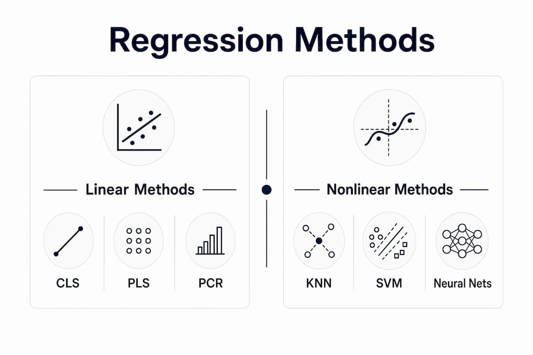
When significant nonlinearities exist, such as scattering effects in diffuse reflectance NIR or matrix interactions in complex biological fluids, kernel-based models like SVR and GPR outperform PLS. The decision between linear and nonlinear methods should be guided by residual analysis, not by visual inspection of spectra alone.
Model comparison must rely on RMSECV and Predictive Residual Sum of Squares (PRESS), not on R² values. R and R² are concentration-range dependent and can appear high even when a model has poor predictive accuracy for samples outside the calibration range. RMSECV gives a direct estimate of prediction error in the same units as the target property, making it the only metric that supports meaningful model comparison.
Pro Tip: Always compare models using RMSECV from cross-validation rather than the calibration R². A model with R² = 0.99 on calibration data but high RMSECV is overfitted and will fail on new samples.
How to ensure quality and representative reference data for reliable regression models?
Reference data quality is the primary determinant of regression model reliability in spectroscopy. No preprocessing pipeline or advanced algorithm compensates for a calibration set that does not represent the operational sample population. The accuracy and range of reference values directly control how well the model generalizes to unknown samples.
The following principles govern effective calibration set design:
- Cover the full operational range. A calibration set that spans only a narrow concentration or property range produces a model with low sensitivity outside that range. The model cannot extrapolate reliably, and predictions for samples near the range boundaries carry disproportionate error.
- Avoid excessive range breadth. A calibration set that spans an unnecessarily wide range forces the model to fit nonlinear behavior that may not exist in the target application. This inflates model complexity without improving practical accuracy.
- Include representative sources of variation. Calibration samples should reflect the temperature, humidity, particle size, and matrix variation that the model will encounter in deployment. Omitting a known source of variation guarantees that the model treats it as prediction error.
- Validate reference measurements independently. Reference values obtained by a single analyst on a single day introduce systematic bias. Cross-laboratory or replicate reference measurements reduce this risk and improve the statistical validity of the calibration.
- Design validation sets separately from calibration sets. Validation samples must come from a different experimental run or time period than calibration samples. Rushing calibration design produces overfitted models that perform well on paper but fail on real-world samples.
Investing time in calibration set design before data collection reduces modeling complexity later and prevents the most common cause of model failure: a calibration set that does not represent the prediction population.
What are the critical validation procedures to confirm a robust spectroscopy regression model?
Validation is the stage where a model either earns scientific credibility or reveals its limitations. A model that has not been validated against an independent sample set has not been validated at all. The following numbered procedure reflects current best practice for spectroscopy regression validation.
-
Cross-validation with RMSECV. Perform leave-one-out or k-fold cross-validation on the calibration set. RMSECV quantifies average prediction error across all held-out samples and guides the selection of the optimal number of PLS components or model hyperparameters.
-
Independent validation set prediction. Apply the final model to a validation set that was not used during calibration or cross-validation. Calculate the Root Mean Square Error of Prediction (RMSEP) and compare it to RMSECV. A large gap between RMSECV and RMSEP indicates overfitting or a calibration set that does not represent the validation population.
-
Bias and slope testing. Regress predicted values against reference values for the validation set. A slope significantly different from 1.0 or an intercept significantly different from 0 indicates systematic model bias that requires investigation.
-
Outlier detection. Calculate leverage and studentized residuals for all calibration and validation samples. High-leverage samples with large residuals distort regression coefficients and should be investigated for measurement error or sample contamination before removal.
-
Reproducibility testing. Repeat predictions on replicate spectra collected on different days or instruments. Reproducibility failure at this stage points to preprocessing inconsistencies or instrument drift that the model has not accounted for.
The table below summarizes the key validation metrics and their interpretation.
| Metric | What it measures | Interpretation |
|---|---|---|
| RMSECV | Cross-validation prediction error | Lower is better; guides component selection |
| RMSEP | Independent validation prediction error | Should be close to RMSECV; large gap signals overfitting |
| PRESS | Sum of squared prediction residuals | Minimized at optimal model complexity |
| Bias | Systematic offset in predictions | Should not differ significantly from zero |
| R² (validation) | Variance explained in validation set | Useful only when combined with RMSEP; not sufficient alone |
R² alone does not confirm model validity in spectroscopy. A model with high R² but poor RMSEP is a calibration artifact, not a predictive tool. Researchers who report only R² values are not providing sufficient evidence for scientific defensibility.
Key takeaways
A defensible spectroscopy regression model requires standardized preprocessing, PLS or nonlinear regression selected on the basis of data characteristics, and validation against an independent sample set using RMSECV and RMSEP rather than R² alone.
| Point | Details |
|---|---|
| Preprocessing sequence matters | Apply baseline correction before smoothing to prevent error propagation across spectral variables. |
| PLS is the standard method | PLS handles collinearity and high dimensionality better than Classical Least Squares for most spectral datasets. |
| Reference data quality drives accuracy | Calibration sets must cover operational variability in range, matrix, and measurement conditions. |
| Use RMSECV, not R², for model selection | RMSECV provides a direct prediction error estimate; R² is concentration-range dependent and misleading. |
| Validate with independent samples | RMSEP from a held-out validation set is the only reliable confirmation of model generalizability. |
Why interpretability is the next frontier in spectral regression
The field has spent two decades refining PLS calibration protocols, and those protocols work. What I find underappreciated is the cost of treating spectral regression as a purely statistical exercise. When a model fails on a new sample batch, the analyst who understands the physical origin of the spectral features can diagnose the problem in minutes. The analyst who only knows the model’s R² value has no starting point.
Interpretable machine learning approaches that combine physical spectral knowledge with statistical modeling are the most productive direction for 2026 and beyond. These hybrid methods do not replace PLS. They add a layer of mechanistic accountability that makes model failures diagnosable rather than mysterious.
The practical implication is that researchers should document which spectral bands drive their regression coefficients, not just the final RMSECV value. That documentation is what separates a model that can be defended in a regulatory submission from one that only works in the lab where it was built. The multivariate analysis methods available today make this documentation feasible without adding significant workflow overhead.
The single most common mistake I observe is rushing the calibration set design to get to the modeling stage faster. The modeling stage is fast. Collecting a well-designed calibration set is slow. Reversing that priority is what produces models that fail six months after deployment.
— Nadeem
R2nsoftware tools for your spectroscopy regression workflow
Researchers who need to move from raw spectral data to validated regression models without rebuilding preprocessing pipelines from scratch will find that R2nsoftware addresses the most time-consuming stages directly.

PeakLab™ supports up to 1,000 peaks simultaneously, resolves overlapping signals that standard fitting routines cannot separate, and integrates baseline modeling directly into the peak analysis workflow. For researchers who need automated preprocessing and signal conditioning before regression modeling, AutoSingal provides standardized signal processing tools designed for spectroscopic data preparation. Both tools produce outputs that feed directly into PLS or nonlinear regression pipelines without manual reformatting. R2nsoftware builds its algorithms on the same mathematical foundations described in this guide, which means the preprocessing outputs are consistent with the validation standards that peer-reviewed spectroscopy requires.
FAQ
What is the best regression method for spectroscopy data?
Partial Least Squares (PLS) is the industry standard for multivariate spectral regression because it handles collinearity and high-dimensional data better than Classical Least Squares. Nonlinear methods like Support Vector Regression are appropriate when scattering or matrix effects create significant nonlinearities.
Why is R² not sufficient for validating a spectroscopy regression model?
R² is concentration-range dependent and does not directly measure predictive accuracy. RMSECV and RMSEP provide direct estimates of prediction error in the units of the target property and are the accepted metrics for model validation.
How many samples are needed for a spectroscopy calibration set?
No universal minimum exists, but the calibration set must cover the full range of the target property and all major sources of spectral variation expected in deployment. Underpopulated calibration sets produce models that overfit and fail on new samples.
What does RMSECV measure in a spectroscopy regression model?
RMSECV is the Root Mean Square Error of Cross-Validation. It estimates the average prediction error across held-out calibration samples and guides selection of the optimal number of model components or hyperparameters.
When should preprocessing include Savitzky-Golay smoothing?
Savitzky-Golay smoothing is appropriate when high-frequency noise is present and peak shape preservation is required for accurate feature extraction. Apply it after baseline correction to avoid spreading baseline artifacts across neighboring spectral points.