
A Guide to 3D Spectral Modeling That Holds Up
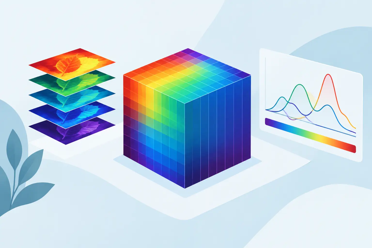
A guide to 3D spectral modeling begins with a practical distinction: a three-dimensional display is not automatically a three-dimensional model. A colored surface, contour plot, or spectral cube can make a complex dataset easier to inspect, but it does not establish which chemical components are present, whether their parameters are identifiable, or whether the result will withstand review. Those questions require a model built around the physics of the measurement, the structure of the data, and explicit statistical validation.
For spectroscopic and analytical datasets, the third dimension may represent time, position, excitation wavelength, emission wavelength, concentration, temperature, or a second instrument response. The resulting data can contain far more information than a sequence of independent 2D traces. It can also multiply the effect of baseline drift, instrumental artifacts, correlated noise, and incorrect assumptions. The objective is not to produce an attractive surface. It is to extract defensible parameters that describe real chemical or physical variation.
What 3D spectral modeling is designed to solve
A 3D spectral dataset is commonly represented as an array with three independent axes. In hyperspectral imaging, those axes may be x position, y position, and wavelength. In a time-resolved experiment, they may be wavelength, signal intensity, and time. Excitation-emission matrices add excitation and emission coordinates, while chromatographic spectral data often combine retention time and wavelength with measured response.
The modeling problem changes with that structure. Fitting each slice independently may be acceptable when spectral shape is known to be invariant and signal-to-noise is high. In many real measurements, it is not. Independent fits can permit peak centers, widths, amplitudes, and baselines to wander from one slice to the next. The result may appear plausible locally while violating known spectral behavior across the full dataset.
A 3D model instead uses the relationships among dimensions. It can enforce shared peak positions, known line-shape behavior, smooth parameter evolution, nonnegative concentrations, or physically justified bounds. Those relationships reduce ambiguity, particularly when peaks overlap or weak components sit on a varying background.
Start with the measurement model, not the visualization
Before selecting an algorithm, define what generated the signal. This is the step that separates scientific modeling from surface approximation.
Ask whether the measured response is additive, multiplicative, or both. A fluorescence intensity surface, for example, may include component emission profiles, excitation dependence, scattering artifacts, detector variation, and baseline contributions. A hyperspectral map may include spatially varying composition, illumination changes, sample topography, and wavelength-dependent response. Treating all of these effects as arbitrary curvature can yield a low residual error while obscuring the actual sample behavior.
The measurement model should identify three elements: the analyte signal, the baseline or background, and the noise process. For peak-resolved spectra, the analyte signal may be represented by Gaussian, Lorentzian, Voigt, Pearson, exponentially modified Gaussian, or other justified line shapes. The correct choice depends on the instrument and underlying physics. A convenient function is not necessarily a valid one.
Baseline terms deserve equal attention. Broad fluorescence, scattering, detector drift, thermal effects, and matrix interference can alter both the apparent amplitude and shape of analyte features. Subtracting a baseline before fitting may be reasonable when the baseline is independently characterized. When it is uncertain or changes across the dataset, simultaneous baseline-and-signal fitting is often the more defensible approach because it preserves the uncertainty and reduces bias in peak parameters.
Prepare the data without erasing the chemistry
Preprocessing should improve model identifiability, not force the data to resemble an expected answer. Start with instrument calibration, axis registration, and inspection for missing values, saturation, spikes, and obvious acquisition artifacts. In a spatial or time-series dataset, misalignment between slices can create artificial broadening and false parameter trends.
Normalization requires similar care. It is useful when the goal is to compare spectral shape independent of total intensity. It is inappropriate when absolute response contains concentration, thickness, path length, or process information. Likewise, smoothing can improve stability in noisy data, but aggressive smoothing may merge adjacent peaks or distort narrow features. Keep the raw data, document every transformation, and verify that preprocessing does not change the interpretation of known standards.
For multidimensional datasets, inspect variation along each axis before fitting the whole array. Plot representative slices from low, medium, and high signal regions. Examine residuals from simple preliminary models. This often exposes changing baselines, saturated regions, or a component that appears only under certain conditions.
Build constraints that reflect real behavior
The strength of 3D spectral modeling lies in its ability to use scientifically justified constraints across the entire dataset. Constraints should be chosen because the experiment supports them, not because they make the optimizer converge.
A peak center may be fixed when a certified standard and calibrated instrument establish its location. It may be allowed to vary within narrow bounds when temperature, composition, or local environment is expected to shift it. Peak widths may be shared across spatial pixels when instrumental broadening dominates, while amplitudes vary with local concentration. In time-resolved work, a smoothness constraint can be appropriate for a parameter expected to change continuously, but not for a reaction that has genuine discontinuities.
Nonnegativity is often essential for component concentrations and intensities. Ratio constraints can be useful for known multiplet structures or isotope patterns. Parameter tying can reduce the number of free variables and improve identifiability, but excessive tying can hide meaningful variation. The correct balance depends on whether a parameter is physically constant, experimentally stable, or merely expected to be similar.
Fit globally when the dimensions share information
Global fitting estimates parameters using the full 3D dataset rather than treating each spectrum, pixel, or time point as an isolated problem. This is especially valuable when individual slices have weak signal, severe overlap, or unstable baselines. Strong features in one region of the dataset can help identify the same component where it is otherwise difficult to resolve.
Several model families may be appropriate. Parametric peak-and-baseline models are well suited to spectra where the components have interpretable positions, widths, and shapes. Multivariate curve resolution can separate evolving component profiles when the number of components and constraints are defensible. Tensor-based methods, including PARAFAC-type approaches, can be useful for trilinear data when their assumptions match the experiment. Surface-fitting methods are appropriate when the target is a continuous response relationship rather than chemical component resolution.
These approaches should not be treated as interchangeable. A smooth fitted surface may describe a calibration response extremely well but provide little evidence about overlapping chemical species. Conversely, a tightly constrained component model may be unsuitable if the data violate its line-shape or trilinearity assumptions. TableCurve Studio can be useful when the scientific question is specifically one of automated 3D surface fitting, but component-resolved spectral interpretation still requires a model that represents the underlying signal structure.
Validate the model beyond residual magnitude
A small residual is necessary but insufficient. Flexible models can fit noise, compensate for a poor baseline with extra peaks, or distribute one physical component across several mathematical terms. Validation must test whether the solution is statistically adequate and scientifically credible.
Examine residual maps across all dimensions. Random, structureless residuals are generally expected after a suitable model has captured the systematic signal. Bands, curved regions, repeated spatial patterns, or time-dependent residual structure indicate a missing component, incorrect baseline treatment, axis misalignment, or unsuitable line shape.
Parameter uncertainty matters as much as parameter estimates. Report confidence intervals, covariance, correlation among fitted parameters, and sensitivity to starting values or reasonable constraint changes. If two overlapping peaks exchange amplitude depending on initialization, the dataset may not identify them separately. The proper response may be to collect higher-resolution data, introduce independent prior information, simplify the model, or report a combined feature rather than an unsupported decomposition.
Use model-selection criteria and cross-validation where applicable, but do not let a single statistic make the decision. The preferred model should improve fit quality without adding parameters that lack physical justification. It should also reproduce known standards, remain stable across replicates, and yield parameters consistent with independent measurements.
Make the workflow reproducible
A defensible 3D spectral result needs a traceable record of the data source, preprocessing choices, model equations, initial conditions, bounds, constraints, optimizer settings, fit statistics, and residual diagnostics. Screenshots of a fitted surface are not sufficient for a publication, quality investigation, or internal technical review.
Create a consistent analysis template for recurring experiments. Use named component definitions, controlled baseline strategies, standardized acceptance criteria, and versioned data exports. For high-throughput work, automated peak detection and optimization can reduce manual repetition, but automation should flag uncertainty and model failure rather than silently return a result for every file.
The most useful 3D spectral model is the one that makes a clear scientific claim and shows why that claim is justified. When the next dataset introduces more overlap, drift, or variation, that discipline gives the model a chance to remain credible rather than merely look convincing.