Genetic Algorithm (Differential Evolution) for Fitting

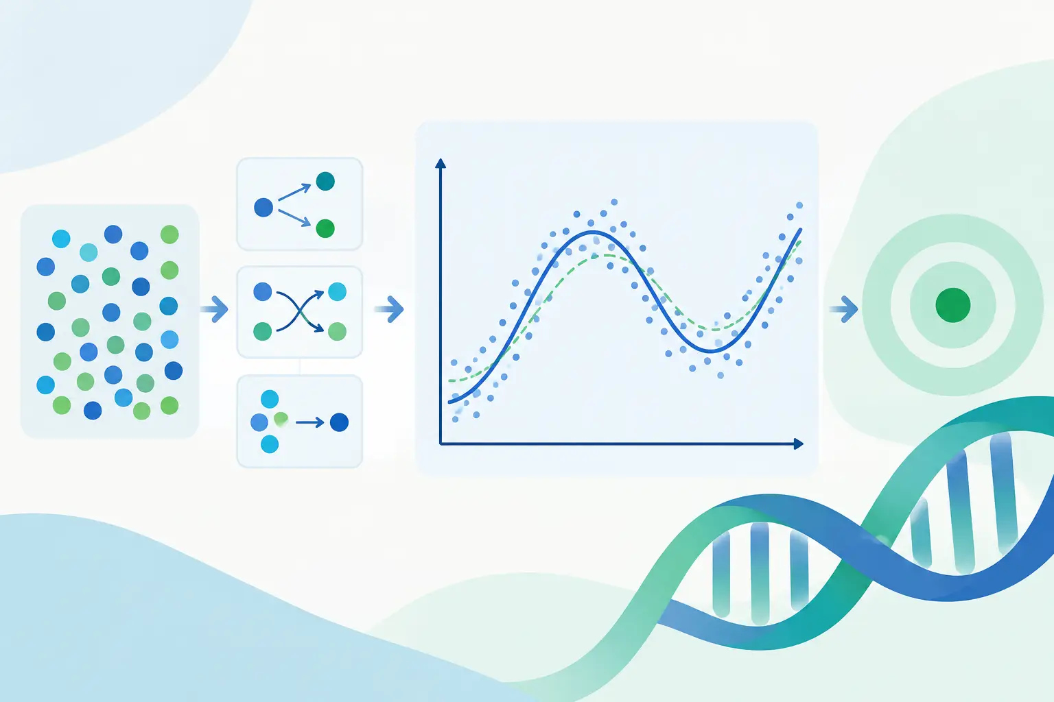
A difficult chromatographic or spectroscopic fit rarely fails because the chosen peak function is unavailable. It fails because the optimizer settles into a mathematically convenient but chemically implausible parameter set. A genetic algorithm (differential evolution) can materially improve this search when overlapping peaks, baseline terms, and constrained nonlinear parameters create an objective surface with many local minima.

Differential evolution is particularly useful when conventional local optimization depends too heavily on initial estimates. It searches a population of candidate solutions across the permitted parameter space, rather than refining only one starting point. For analytical scientists, that distinction matters when a visually acceptable fit can conceal swapped peak assignments, unrealistic widths, negative amplitudes, or a baseline that absorbs analyte signal.

What Differential Evolution Actually Does

Differential evolution is an evolutionary optimization method. It is often grouped with genetic algorithms because it evolves a population through repeated candidate generation, selection, and replacement. Strictly speaking, it differs from many classical genetic algorithms: its defining operation uses scaled differences between population members to generate new trial vectors, rather than relying primarily on binary encoding and crossover.

Each candidate vector represents a complete set of model parameters. In a peak-fitting problem, that vector may include peak centers, heights or areas, widths, asymmetry terms, baseline coefficients, and response-model parameters. The optimizer evaluates each vector against an objective function, commonly a weighted residual sum of squares. Candidates that reduce the objective function survive into the next generation.

The method is governed by practical controls: population size, differential weight, crossover probability, parameter bounds, and stopping criteria. These settings affect search coverage, computational cost, and the likelihood of locating a useful basin of attraction. There is no universal configuration. A narrow, well-characterized Gaussian peak set and a strongly overlapping asymmetric multiplet should not be treated as the same optimization problem.

Why a Genetic Algorithm (Differential Evolution) Helps

Nonlinear fitting becomes difficult when parameters are correlated. Peak width and amplitude can compensate for one another. A drifting baseline can trade off against broad low-intensity features. Neighboring peak centers can move in opposite directions while producing nearly the same composite curve. Local algorithms such as Levenberg-Marquardt are highly efficient near the correct solution, but they can converge to the nearest acceptable basin rather than the scientifically correct one.

Differential evolution addresses the initialization problem by searching broadly within defined bounds. It can test parameter combinations that an analyst would not reasonably supply as manual starting estimates. That is valuable in automated or high-throughput workflows, where hundreds of data files cannot receive extensive hand tuning.

Its value is strongest in several situations:

• severely overlapping peaks with uncertain initial centers or widths;
• models that combine nonlinear baseline and peak parameters;
• asymmetric, Voigt, exponentially modified, or otherwise complex line shapes;
• surface-fitting and multidimensional models with a large search space;
• batch analysis where reproducible search rules matter more than operator-specific starting guesses.

The advantage is not that differential evolution eliminates scientific judgment. It moves the initial global search from ad hoc guessing to a defined, repeatable procedure. The analyst still determines which model family is physically credible, which parameters may vary, and what limits are scientifically justified.

Bounds and Constraints Determine Whether the Result Is Defensible

An unconstrained global optimizer is not inherently a better optimizer. Given enough freedom, it can identify parameter sets that lower residual error while violating instrument physics, chemistry, or known process behavior. A negative concentration proxy, an impossible retention order, or a peak width exceeding the relevant separation scale may improve a numerical criterion while weakening the interpretation.

For that reason, parameter bounds are not merely computational safeguards. They encode prior scientific knowledge. Centers can be limited to expected spectral or retention regions. Widths can be constrained to realistic instrument resolution. Peak areas can be required to remain nonnegative. Shared parameters can be imposed when replicate signals are expected to have a common width, response factor, or line-shape component.

Constraints also reduce an optimizer’s ability to exchange one physical explanation for another. In deconvolution, for example, a broad baseline component should not be permitted to mimic a known unresolved analyte band without scrutiny. In multichannel spectroscopy, linked peak positions or widths may be more defensible than allowing each trace to fit independently.

The appropriate degree of constraint depends on the application. Exploratory research may begin with wider bounds to expose unexpected structure. A validated quality-control method generally requires tighter, predefined limits and documented exception handling. In either case, every constraint should be traceable to a scientific, instrumental, or method-development rationale.

Global Search Should Usually Be Followed by Local Refinement

Differential evolution is effective at locating promising regions of parameter space, but it is not always the most efficient final estimator. Population-based search requires many objective-function evaluations. This cost grows quickly when fitting dense spectra, large chromatographic batches, or high-dimensional surfaces.

A hybrid workflow is often the stronger approach. Differential evolution first identifies a credible global candidate within the required bounds. A local nonlinear least-squares method then refines that candidate to improve parameter precision and convergence efficiency. The final calculation should use appropriate residual weighting, scaling, and convergence tolerances for the data and measurement model.

This sequence also clarifies the respective roles of the algorithms. Differential evolution answers, “Where is the plausible solution region?” Local refinement answers, “What are the best parameter estimates within that region?” Treating them as complementary methods is more productive than presenting one as a replacement for the other.

For repeated workflows, reproducibility requires more than retaining the final fitted curve. The software environment should record the model definition, parameter bounds, constraints, objective function, optimization settings, random seed or reproducibility policy, and final convergence status. Without this information, a result may be difficult to reproduce even when the raw data are available.

Residuals Still Decide Whether the Model Is Adequate

A low sum of squares is not proof that the fitted components are valid. Differential evolution can locate a lower minimum than a manually initialized local search, yet the resulting model may still be overparameterized or physically unconvincing. Fit evaluation must extend beyond visual overlay.

Residual plots should be inspected for structured departures, especially around peak shoulders, inflection regions, and baseline transitions. Randomly distributed residuals are generally more consistent with an adequate model than repeating positive-negative patterns. Analysts should also examine parameter confidence intervals, covariance or correlation structure, residual standard deviation, reduced chi-square where applicable, information criteria for competing models, and consistency across replicate measurements.

Parameter correlation deserves particular attention. Two components may produce a stable composite curve while their individual areas or widths remain poorly identifiable. This is common with closely overlapping features. Reporting component-specific quantities without recognizing uncertainty can overstate what the data support.

The number of fitted peaks should likewise be based on chemical knowledge, orthogonal measurements, expected retention or spectral positions, and statistically meaningful model comparison. An optimizer cannot determine whether an apparent shoulder is a new chemical species, baseline artifact, detector disturbance, or noise. It only optimizes the model it is given.

Practical Use in Peak and Surface Modeling

For analytical datasets, the most productive use of differential evolution is targeted rather than indiscriminate. Begin with preprocessing that preserves the information needed for modeling: correct import of instrument data, appropriate handling of missing points, and a baseline strategy consistent with the measurement process. Define a line shape supported by the physics and by observed residual behavior. Then establish bounded, interpretable parameters before global optimization begins.

In a complex peak-fitting workflow, the optimizer may search centers, widths, amplitudes, and baseline terms jointly. That can outperform a sequential approach when baseline and peak parameters are strongly coupled. However, joint fitting also increases dimensionality and the possibility of nonidentifiable solutions. A staged procedure may be preferable when baseline regions are well established or when selected parameters can be fixed from calibration data.

For automated curve and surface fitting, the same principle applies. Differential evolution can identify viable starting regions for nonlinear equations whose parameters have non-obvious interactions. It should not be used to compensate for an unsuitable equation, unscaled variables, or an absence of experimentally meaningful bounds.

R²N Software applies this perspective to professional analytical modeling: optimization is valuable when it supports interpretable parameters, statistically reliable diagnostics, and methods that can be defended beyond a graphically convincing overlay.

The practical standard is straightforward: use differential evolution to search broadly when the problem warrants it, then require the final model to earn trust through constraints, residual evidence, uncertainty analysis, and reproducible reporting.