How Monte Carlo Simulation Supports Statistical Analysis

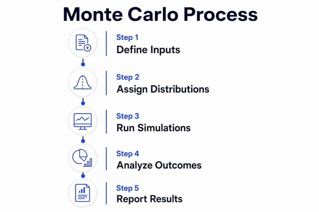
Monte Carlo simulation is a computational method that replaces fixed inputs with probability distributions and uses repeated random sampling to generate a full distribution of possible outcomes. Each iteration draws new random values, evaluates the model, and stores the result. After thousands of runs, analysts examine percentiles, risk probabilities, and tail behaviors that a single deterministic estimate cannot reveal. Tools like @RISK and ANSYS apply this method across engineering, finance, physics, and biotechnology. Understanding how Monte Carlo simulation supports analysis means understanding how probabilistic thinking replaces false certainty with calibrated, defensible insight.
How Monte Carlo simulation supports analysis through uncertainty quantification
Single-point forecasts produce a single answer. Monte Carlo produces a distribution of answers, each weighted by the probability of its underlying inputs occurring together. That shift from one number to a full probability curve is the core benefit of the method.
Practitioners analyze percentiles like P10, P50, and P90 to understand the spread of likely outcomes. P50 represents the median outcome. P10 and P90 bound the range where 80% of results fall, giving decision-makers a calibrated view of best-case and worst-case scenarios without requiring them to guess.
Monte Carlo simulation benefits are most visible in budgeting and scheduling contexts. A project manager using Monte Carlo does not ask “will we finish on time?” but rather “what is the probability we finish within 12 months?” That reframing produces answers that support resource allocation, contingency planning, and stakeholder communication.
- Probability of threshold exceedance: Analysts calculate the probability that cost exceeds a budget cap or that a process variable crosses a safety limit.
- Percentile-based targets: P50 serves as the expected outcome; P90 sets a conservative planning target with only a 10% chance of being exceeded.
- Risk tolerance evaluation: Stakeholders select acceptable probability thresholds and trace them back to required inputs or design margins.
- Distribution selection: Inputs modeled as triangular, normal, lognormal, or PERT distributions reflect real-world variability more accurately than fixed values.
Pro Tip: When selecting input distributions, use historical data or expert elicitation to set distribution parameters. A poorly chosen distribution shape introduces more error than a small sample size.
The output of a Monte Carlo run is not a recommendation. It is a map of the probability space. Analysts interpret that map relative to organizational risk tolerance, regulatory thresholds, or performance specifications.
How does Monte Carlo support sensitivity analysis?
Sensitivity analysis identifies which uncertain inputs drive the most variability in outputs. Monte Carlo simulation supports global sensitivity analysis by decomposing output variance across all inputs simultaneously, rather than varying one input at a time while holding others fixed.

The one-at-a-time approach misses interaction effects. When two inputs jointly affect an output in a non-additive way, one-at-a-time testing assigns credit incorrectly. Global methods like Sobol indices capture these interactions and rank inputs by their total contribution to output variance.
The practical result is a ranked list of uncertainty drivers. Analysts use that list to focus mitigation resources on the variables that matter most. A variable ranked low in Sobol indices does not warrant expensive data collection or tighter process control.
- Run the Monte Carlo model with all uncertain inputs active and collect output distributions.
- Compute Sobol first-order indices to measure each input’s direct contribution to output variance.
- Compute total-order indices to capture each input’s contribution including all interaction effects with other variables.
- Rank inputs by total-order index and identify the top two or three drivers of output uncertainty.
- Focus mitigation on top-ranked inputs by reducing their uncertainty through better data, tighter tolerances, or process controls.
Pro Tip: Tornado charts visualize one-at-a-time sensitivity quickly, but always follow up with Sobol indices for models with more than three uncertain inputs. Tornado charts can rank drivers incorrectly when interactions are present.
Combining Monte Carlo with global sensitivity methods transforms a probabilistic model from a passive forecasting tool into an active guide for model improvement and risk control. That combination is what separates rigorous uncertainty quantification from simple scenario testing.
Monte Carlo vs. scenario analysis: handling complex, non-linear systems
Scenario analysis evaluates a small number of discrete cases, typically best, base, and worst. Monte Carlo evaluates the full joint effect of all uncertain inputs simultaneously across thousands of combinations. The difference is not cosmetic. It is structural.
Complex systems exhibit non-linear responses. A 10% increase in one input combined with a 5% decrease in another may produce an output change that neither effect predicts alone. Scenario analysis misses those combinations unless they are explicitly constructed. Monte Carlo samples the full joint distribution and captures them automatically.
| Method | Inputs evaluated | Interaction effects | Output format | Typical use case |
|---|---|---|---|---|
| Scenario analysis | 3–5 discrete cases | Not captured | Single values per scenario | Strategic planning, communication |
| One-at-a-time sensitivity | One variable at a time | Not captured | Ranked list | Simple linear models |
| Monte Carlo simulation | Full joint distribution | Fully captured | Probability distribution | Risk analysis, engineering, research |
The table above shows why Monte Carlo is the preferred method for systems where inputs interact. Engineering models for structural reliability, pharmacokinetic models in biotechnology, and financial portfolio models all exhibit non-linear behavior that scenario analysis cannot adequately characterize.
ANSYS documents Monte Carlo applications across engineering and physics where input uncertainties propagate through complex governing equations. In those contexts, a three-scenario analysis would miss the tail risks that drive design decisions.
The method also bridges qualitative risk identification and quantitative probabilistic risk analysis. Risk registers identify uncertain variables. Monte Carlo assigns distributions to those variables and quantifies their combined effect on project or system outcomes.
What industries use Monte Carlo simulation effectively?
Monte Carlo simulation is applied wherever uncertain inputs feed into models with consequential outputs. The method is not domain-specific. Its value scales with the complexity and consequence of the decision being supported.
- Engineering and reliability: Structural analysts propagate material property uncertainties through finite element models to estimate failure probabilities under load. ANSYS and similar platforms support this workflow natively.
- Finance and portfolio analysis: Risk managers model correlated asset returns to estimate value-at-risk and expected shortfall across thousands of market scenarios.
- Physics and chemistry: Researchers propagate measurement uncertainty through reaction kinetics models or particle transport simulations to characterize output confidence intervals.
- Biotechnology and clinical research: Pharmacokinetic modelers use Monte Carlo to propagate patient variability through dose-response models, supporting regulatory submissions.
- Project management: Schedule and cost analysts apply Monte Carlo to quantify the probability of on-time, on-budget delivery given uncertain task durations and resource availability.
Reliable outputs require sufficient iterations. Sampling error decreases with the square root of the number of runs, meaning doubling iterations reduces error by a factor of roughly 1.41. Analysts targeting stable P90 estimates typically run 10,000 or more iterations depending on model complexity.
Correlated inputs require careful modeling using dependence-preserving sampling techniques. Ignoring correlations between uncertain variables produces joint scenarios that cannot occur in reality, distorting risk band estimates and leading to incorrect prioritization.
A recommended workflow follows four steps: fit distributions to data, validate the model against observed outcomes, run Monte Carlo for output characterization, then apply global sensitivity analysis to identify which inputs drive tail behavior. This calibration and validation sequence ensures that probabilistic outputs reflect the actual system rather than modeling assumptions.
Key Takeaways
Monte Carlo simulation supports analysis by replacing single-point estimates with probability distributions, enabling quantified uncertainty, ranked sensitivity, and probabilistic decision-making across engineering, finance, and scientific research.
| Point | Details |
|---|---|
| Probabilistic output over point estimates | Monte Carlo generates full output distributions, enabling P10, P50, and P90 analysis instead of a single forecast value. |
| Global sensitivity analysis | Sobol indices rank uncertain inputs by their total contribution to output variance, including interaction effects missed by one-at-a-time methods. |
| Non-linear system handling | Monte Carlo evaluates the full joint distribution of inputs simultaneously, capturing interaction effects that scenario analysis cannot. |
| Iteration count matters | Sampling error decreases with the square root of runs; stable P90 estimates typically require 10,000 or more iterations. |
| Correlated inputs need explicit modeling | Ignoring input correlations distorts joint scenarios and produces inaccurate risk band estimates. |
Why most analysts underuse Monte Carlo’s full capability
The method is widely known. Its full analytical potential is less commonly realized. Most analysts run Monte Carlo to get a P50 estimate and stop there. That approach uses roughly 20% of what the method offers.
The real value sits in the tails and in the sensitivity decomposition. P90 and P95 estimates reveal the scenarios that drive contingency budgets, safety margins, and regulatory limits. Sobol indices reveal which inputs control those tails. Without that second step, analysts know that risk exists but cannot say where to focus.
I have seen teams run 1,000-iteration models and trust the P90 output without checking convergence. That is a structural error. The P90 of a 1,000-run model can shift meaningfully with a different random seed. Running convergence diagnostics before reporting tail estimates is not optional. It is part of the method.
The other underused capability is correlation modeling. Real systems have correlated inputs. Material strength and density correlate. Project task durations correlate within work packages. Treating those inputs as independent inflates the apparent uncertainty range and misidentifies risk drivers. Dependence-preserving sampling techniques like Iman-Conover or copula-based methods address this directly.
The mindset shift that makes Monte Carlo genuinely useful is treating uncertainty as first-class information rather than noise to be eliminated. A well-calibrated probability distribution tells you more than a confident point estimate. Analysts who internalize that principle extract far more decision-relevant insight from the same model.
— Nadeem
R2nsoftware tools for probabilistic analysis workflows
Analysts who work with spectroscopic, chromatographic, or signal-rich datasets face a specific challenge: uncertainty in peak parameters propagates through every downstream calculation. R2nsoftware’s PeakLab addresses this directly by applying advanced mathematical algorithms and statistical models to characterize peaks, baselines, and overlapping signals with scientifically defensible precision.

PeakLab supports up to 1,000 simultaneous peaks, enabling analysts to resolve overlapping signals that standard tools cannot separate. That resolution quality directly improves the reliability of input distributions fed into Monte Carlo workflows. R2nsoftware also provides video resources demonstrating analytical workflows, including uncertainty quantification and sensitivity analysis applications relevant to chromatography and spectroscopy researchers.
FAQ
What is Monte Carlo simulation in statistical analysis?
Monte Carlo simulation is a method that replaces fixed model inputs with probability distributions and uses repeated random sampling to generate a full distribution of possible outputs. Analysts use the resulting percentiles and probabilities to quantify uncertainty and support decisions.
How does Monte Carlo simulation differ from scenario analysis?
Scenario analysis evaluates a small number of discrete input combinations. Monte Carlo samples the full joint distribution of all uncertain inputs simultaneously, capturing interaction effects and tail risks that scenario analysis cannot represent.
How many iterations does a Monte Carlo simulation need?
Sampling error decreases with the square root of the number of iterations. Stable estimates at the P90 level typically require 10,000 or more runs, depending on model complexity and the precision required for tail estimates.
What is sensitivity analysis in Monte Carlo simulation?
Sensitivity analysis within Monte Carlo ranks uncertain inputs by their contribution to output variability. Global methods like Sobol indices decompose output variance across all inputs simultaneously, including interaction effects, and identify the key drivers of risk.
Why do correlated inputs matter in Monte Carlo simulation?
Ignoring correlations between uncertain inputs produces joint scenarios that cannot occur in reality. Dependence-preserving sampling techniques model these correlations correctly, improving the accuracy of risk band estimates and variable prioritization.