
Multivariate Statistical Analysis of Spectra: 2026 Guide

Multivariate statistical analysis of spectra is defined as the application of chemometric and mathematical methods to simultaneously interpret multiple correlated spectral variables, extracting chemical and structural information that univariate approaches cannot resolve. Spectral measurements are inherently multivariate because chemical samples produce overlapping signals across hundreds or thousands of wavelengths, mass-to-charge ratios, or frequency bins. Methods including Principal Component Analysis (PCA), Partial Least Squares Regression (PLSR), and Multivariate Curve Resolution with Alternating Least Squares (MCR-ALS) each address a distinct analytical challenge within this framework. Applying the right technique to the right problem determines whether your model produces defensible chemical insight or a statistically plausible artifact.
Which multivariate statistical techniques work best for spectral data?
Core multivariate techniques for spectral data divide into three functional categories: dimensionality reduction, predictive calibration, and signal deconvolution. Each category maps to a specific analytical objective, and selecting the wrong category is the most common source of misinterpretation in spectral studies.
Principal Component Analysis reduces high-dimensional spectral data to a smaller set of orthogonal components that capture maximum variance. In practice, PCA scores plots reveal sample clustering by chemical class, while loadings plots identify which spectral regions drive that separation. PCA does not require a reference concentration value, making it the standard first step for exploratory analysis of mass spectrometry datasets.

Partial Least Squares Regression builds calibration models that relate spectral variation directly to a measured property, such as analyte concentration or reaction yield. PLSR handles collinear spectral variables without the instability that ordinary least squares regression produces under those conditions. It is the method of choice when you need quantitative prediction from spectra with overlapping absorption bands.
MCR-ALS resolves a mixture spectrum into contributions from individual pure components using iterative least squares optimization under chemical constraints such as non-negativity. The mcrpure approach identifies pure spectral variables and decomposes the data matrix into concentration profiles and pure component spectra. MCR-ALS is indispensable for time-resolved or spatially resolved spectral datasets where component identities are unknown.
Thomson’s Multitaper Method (MTM) addresses spectral density estimation rather than chemometric modeling. MTM achieves K-fold lower variance than raw periodograms by averaging estimates from multiple orthogonal Slepian tapers. This makes it the preferred non-parametric tool for detecting periodic signals in noisy spectral time series.
| Method | Primary Use | Key Strength | Limitation |
|---|---|---|---|
| PCA | Dimensionality reduction | No reference values needed | Unsupervised; no prediction |
| PLSR | Quantitative calibration | Handles collinear variables | Requires reference measurements |
| MCR-ALS | Component deconvolution | Resolves unknown mixtures | Sensitive to initial estimates |
| MTM | Spectral density estimation | Low-variance frequency estimates | Not suited for concentration modeling |
Pro Tip: Run PCA before PLSR on every new dataset. The scores plot will reveal outliers and batch effects that would otherwise corrupt your calibration model without warning.
How should you preprocess spectral data before multivariate analysis?
Preprocessing is not optional. Raw spectral data fed directly into multivariate models produces results that reflect instrument drift, concentration differences, and baseline offsets rather than true chemical composition.
Normalization is the single most consequential preprocessing decision. Failing to normalize spectral data causes clustering driven by sample concentration rather than spectral shape, which renders PCA scores plots chemically meaningless. Normalization to unit area or maximum absorbance forces the model to compare spectral profiles on equal footing.
Variable selection reduces the dimensionality of the input matrix before modeling, removing spectral regions that carry no chemical information. The combination of Wavelet Packet Transform with Modified Uninformative Variable Elimination (WPT-MUVE) outperforms standard PLS in calibration accuracy by removing redundant variables prior to model construction. This approach was validated on milk powder component analysis, where spectral overlap between fat, protein, and lactose bands is severe.
Baseline correction removes broad, slowly varying background signals that shift the spectral baseline across samples. Robust background estimation using LOWSPEC combined with multitaper methods improves signal detection in noisy spectra by applying locally weighted regression to model the spectral background before analysis.
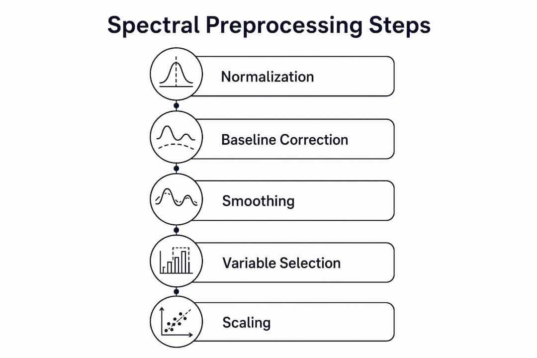
A complete preprocessing sequence should include:
- Spectral smoothing or noise filtering (Savitzky-Golay or wavelet denoising)
- Baseline correction using LOWSPEC, asymmetric least squares, or polynomial fitting
- Normalization to unit area, maximum absorbance, or total ion current for mass spectrometry
- Variable selection using WPT-MUVE or interval PLS to remove uninformative spectral regions
- Outlier detection via Hotelling’s T² and Q-residuals from an initial PCA model
Pro Tip: Apply normalization before baseline correction when your baseline shifts are concentration-dependent. Reversing this order can introduce systematic error that propagates through every downstream model.
Step-by-step workflow for multivariate spectral analysis
A reproducible workflow prevents the most common failure mode in spectral chemometrics: building a model that fits the training set but fails on independent validation samples.
- Design the experiment before collecting data. Define the analyte range, sample matrix, and expected sources of spectral variation. An underpowered calibration set produces a PLSR model that cannot generalize.
- Acquire and format the data matrix. Organize spectra as rows and spectral variables as columns. For mass spectrometry data, align spectra to a common m/z axis before any statistical processing.
- Execute the preprocessing sequence. Apply smoothing, baseline correction, normalization, and variable selection in the order established during experimental design.
- Run PCA and inspect scores and loadings. Identify the number of significant principal components using a scree plot or cross-validation. Loadings plots identify which spectral features drive sample separation.
- Build the PLSR calibration model. Use leave-one-out or k-fold cross-validation to select the optimal number of latent variables. Report root mean square error of cross-validation (RMSECV) and root mean square error of prediction (RMSEP) on an independent test set.
- Apply MCR-ALS for mixture resolution. Initialize with pure variable estimates from mcrpure or singular value decomposition. Apply non-negativity constraints on both concentration profiles and spectra. Assess lack of fit and explained variance at convergence.
- Interpret nonlinear models with explainable AI. Machine learning models for spectral data require XAI techniques to confirm that feature importance scores reflect genuine chemical signals rather than data artifacts.
| Step | Method | Output |
|---|---|---|
| Preprocessing | WPT-MUVE, LOWSPEC, normalization | Clean, scaled spectral matrix |
| Exploration | PCA | Scores, loadings, outlier flags |
| Calibration | PLSR | Concentration predictions, RMSEP |
| Deconvolution | MCR-ALS | Pure component spectra and profiles |
| Validation | Cross-validation, permutation tests | Model reliability metrics |
R2nsoftware’s PeakLab supports up to 1,000 simultaneous peaks with integrated baseline modeling, making it directly applicable at steps 3 and 6 of this workflow.
Pro Tip: Always report RMSEP on samples collected on a different day than the calibration set. Same-day validation inflates model performance and conceals instrument drift effects.
How do you validate and troubleshoot multivariate spectral models?
Validation is where most spectral chemometrics projects either earn credibility or collapse. Statistical fit metrics alone are insufficient. A model must also make chemical sense.
Overfitting is the most frequent error. A PLSR model with too many latent variables will fit calibration noise and fail on new samples. Cross-validation RMSECV that is substantially lower than RMSEP on an independent set is the diagnostic signal. Reduce the number of latent variables until the gap closes.
Permutation testing provides a distribution-free check on model significance. Permutation-based methods like PERMANOVA avoid strict parametric assumptions and are applicable to complex experimental designs where normality cannot be assumed. Running 999 permutations of the class labels and comparing the observed F-statistic to the permuted distribution confirms whether group separation in PCA or discriminant analysis is statistically real.
Clustering artifacts from normalization errors are a persistent problem. Normalization errors in spectral data produce artificial clusters that reflect scaling choices rather than chemical differences. Always rerun PCA with and without normalization to confirm that observed clusters are not normalization artifacts.
Chemical validation must accompany every statistical conclusion. Machine learning feature importance scores can highlight data artifacts rather than true chemical signals. Treat every feature importance result as a hypothesis and verify it against known spectroscopic assignments or reference standards.
Troubleshooting checklist for multivariate spectral models:
- Confirm normalization was applied before modeling, not after
- Check that the number of PLSR latent variables was selected by cross-validation, not by training set R²
- Verify MCR-ALS convergence by inspecting residual spectra for systematic structure
- Run permutation tests to confirm statistical significance of group separation
- Cross-reference spectral loadings with published band assignments for the analyte system
- Test model performance on samples from a different instrument or operator
Pro Tip: When MCR-ALS residuals show a systematic peak at a specific wavelength, that peak is almost always a component you did not include in the initial model. Add it rather than ignoring it.
Key takeaways
Reliable multivariate spectral analysis requires matched method selection, rigorous preprocessing, and chemical validation at every modeling stage.
| Point | Details |
|---|---|
| Match method to objective | Use PCA for exploration, PLSR for calibration, and MCR-ALS for component deconvolution. |
| Normalize before modeling | Skipping normalization causes concentration-driven clustering that misrepresents chemical composition. |
| Validate on independent data | Report RMSEP on samples collected separately from the calibration set to expose drift and overfitting. |
| Use permutation tests | PERMANOVA and related methods confirm group separation without requiring normality assumptions. |
| Treat XAI outputs as hypotheses | Feature importance scores from nonlinear models require independent chemical verification before interpretation. |
Where chemometrics meets chemical reality
My view on multivariate spectral analysis has shifted considerably over the past decade, and not in the direction most software vendors would prefer. The field has moved fast toward nonlinear machine learning models, and the results are genuinely impressive on benchmark datasets. The problem is that benchmark datasets are not your dataset.
The transition from linear chemometric models to nonlinear machine learning requires new validation frameworks that most laboratories have not yet built. I have seen SHAP values and gradient-based attribution maps presented as chemical evidence in peer-reviewed manuscripts, when the underlying model was trained on 40 samples with 4,000 spectral variables. That is not chemometrics. That is overfitting with a visualization layer on top.
The preprocessing innovations that genuinely move the needle are less glamorous. WPT-MUVE variable selection and robust background estimation with LOWSPEC are not headline features, but they consistently produce more transferable models than any nonlinear architecture applied to raw data. The researchers who understand this distinction produce work that holds up under external validation.
My practical advice: build your PLSR or MCR-ALS model first. If it fails to meet your accuracy requirements after rigorous preprocessing and cross-validation, then consider a nonlinear approach with explainable AI transparency built in from the start. Do not start with complexity. Complexity is where chemical plausibility goes to die.
— Nadeem
How R2nsoftware supports spectral analysis workflows
R2nsoftware builds tools specifically for researchers who need mathematical rigor at every stage of spectral data analysis. PeakLab™ handles up to 1,000 simultaneous peaks with advanced baseline modeling and Voigt deconvolution, directly supporting the preprocessing and component resolution steps described in this guide.

For signal analysis tasks including spectral density estimation and noise separation, AutoSingal provides dedicated algorithms that complement multivariate workflows. The R2nsoftware video tutorial library covers practical applications of peak fitting, baseline correction, and curve fitting for spectroscopy and chromatography researchers. If you are building or refining a multivariate spectral analysis pipeline, the PeakLab product page details the full capability set with documented methodology.
FAQ
What is multivariate statistical analysis of spectra?
Multivariate statistical analysis of spectra is the application of chemometric methods such as PCA, PLSR, and MCR-ALS to interpret multiple correlated spectral variables simultaneously. It extracts chemical information that single-wavelength or univariate analysis cannot resolve.
When should you use PCA vs. PLSR for spectral data?
Use PCA when your goal is exploratory pattern recognition or outlier detection without reference concentration values. Use PLSR when you need quantitative prediction of a chemical property from spectral measurements.
How does normalization affect multivariate spectral models?
Normalization to unit area or maximum absorbance forces the model to compare spectral shapes rather than concentration magnitudes. Without it, clustering and classification results reflect sample loading rather than chemical composition.
What is mcr-als used for in spectroscopy?
MCR-ALS resolves a measured mixture spectrum into pure component spectra and concentration profiles using iterative least squares under non-negativity constraints. It is applied when component identities are unknown and spectral overlap prevents direct assignment.
How do you confirm a multivariate spectral model is statistically valid?
Report RMSEP on an independent test set and run permutation tests such as PERMANOVA to confirm that group separation exceeds chance. Cross-validation on the training set alone is insufficient for publication-quality validation.