TableCurve 3D
When the response depends on two things at once, a curve will not tell you about it. TableCurve 3D fits more than 38,000 surface equations to your XYZ data and ranks them the same way the 2D engine ranks curves — then lets you turn the surface around and look at it from any angle.
38,000 surfaces, sorted for you
Surface fitting is where guessing a model breaks down completely. The interaction between two variables rarely looks like anything you would nominate by eye, and the difference between a saddle, a ridge and two separate modes is not something a contour plot settles. So the engine fits the library and lets the statistics argue.
Ranked surface fits
The full surface library is fitted and scored on r², adjusted r², the F-statistic and standard error, exactly as in the 2D engine.
Contours and projections
Every fitted surface comes with contour and density views. Reading level curves is often how a mechanism becomes obvious.
Rotate and animate
Spin the surface live to check whether a feature is real structure or an artefact of the viewing angle, and record the rotation for a presentation.
Gridding for scattered data
Real measurements rarely land on a neat lattice. Scattered XYZ points are gridded before fitting so irregular sampling is not a barrier.
Your own surfaces
Enter a function of x and y in algebraic notation and it is fitted and ranked beside the built-in library.
Publication output
Surfaces, contours, coefficient tables and the statistical summary export to Word and Excel at presentation resolution.
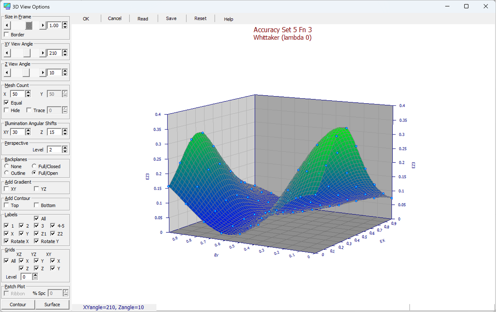
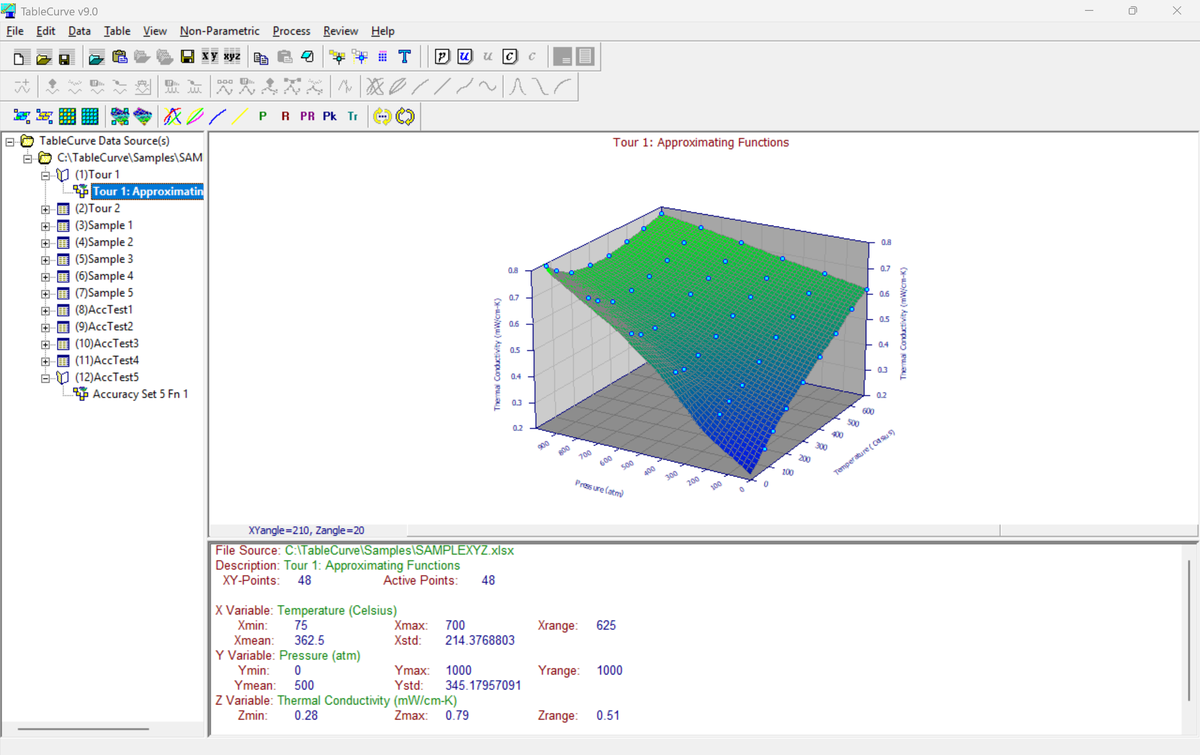
Surfaces drawn by the fitting engine
Captures from TableCurve 9 itself. Shading, mesh density, view angle, backplanes and contour overlays are all set from the panel beside the graph.
Four steps from scattered points to a surface
-
Bring in XYZ
Three columns, however they were sampled. Paste, open a file, or type them in.
-
Grid and fit
Scattered points are gridded, then the selected surface families are fitted and scored.
-
Look from every angle
Rotate the ranked surfaces, switch to contours, and check the residuals across the plane.
-
Take the model out
Export the surface, the contour map, the coefficients or generated source code.
What is in the box
TableCurve 3D is the XYZ half of the TableCurve 9 program. It installs and licenses on its own, and upgrades to Studio by changing the licence key rather than the installation.
A 3D licence can open and view 2D functions, but curve fitting requires TableCurve 2D or Studio.
- Data model
- XYZ triples, two independent variables
- Equations
- 38,000+ built-in surfaces, plus user-defined functions
- Preprocessing
- Gridding and smoothing for scattered or irregular sampling
- Precision
- 128-bit extended-precision solver for ill-conditioned fits
- Statistics
- r², adjusted r², F-statistic, standard error, coefficient confidence intervals
- AI guidance
- Copy for Claude.ai — hands over the equation, statistics and residuals
- Graphics
- Rotatable surfaces, contour and density maps, residual surfaces
- Export
- Word, Excel, clipboard, generated source code
- Platform
- Windows 10 and 11, 64-bit
- Licensing
- Annual or perpetual, academic or commercial
Find out what your second variable is doing
The trial fits the full surface library. Load the experiment you have been treating as two separate curves and see what it looks like as one surface.